Discrete Probability Distributions: Study Notes

Discrete Probability Distributions

Probability Distributions

A probability distribution describes how probabilities are distributed over the values of a random variable. In statistics, random variables can be either discrete or continuous, and their probability distributions differ accordingly.

• Random Variable: A variable that represents a numerical value associated with each outcome of a probability experiment. Denoted by x.

• Discrete Random Variable: Has a finite or countable number of possible outcomes (e.g., number of sales calls in a day).

• Continuous Random Variable: Has an uncountable number of possible outcomes, represented by an interval on the number line (e.g., hours spent on sales calls).

Example: The number of Fortune 500 companies that lost money in the previous year is a discrete random variable because it can be counted. The volume of gasoline in a 21-gallon tank is a continuous random variable because it can take any value within an interval.

Constructing a Discrete Probability Distribution

A discrete probability distribution lists each possible value the random variable can assume, together with its probability. The distribution must satisfy two conditions:

• Each probability is between 0 and 1, inclusive.

• The sum of all probabilities is 1.

Steps to Construct:

1. List all possible outcomes of the discrete random variable.

2. Make a frequency distribution for these outcomes.

3. Find the sum of the frequencies.

4. Calculate the probability for each outcome: Probability = (Frequency of outcome) / (Total frequency).

5. Check that all probabilities are between 0 and 1 and that their sum is 1.

Example: An industrial psychologist administered a personality inventory test for passive-aggressive traits to 150 employees, scoring from 1 (extremely passive) to 5 (extremely aggressive). The probability distribution is constructed by dividing the frequency of each score by 150.

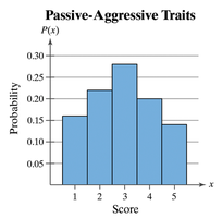
The histogram above shows the probability distribution for the scores. The distribution is approximately symmetric, and the area of each bar represents the probability of each outcome.

Verifying a Probability Distribution

To verify if a distribution is a valid probability distribution, ensure:

• Each probability is between 0 and 1, inclusive.

• The sum of all probabilities equals 1.

Example: If the sum of probabilities is greater than 1 or if any probability is negative or greater than 1, the distribution is not valid.

Mean of a Discrete Probability Distribution

The mean (or expected value) of a discrete probability distribution is calculated as:

$\mu = \sum [x \cdot P(x)]$

• Multiply each value of x by its probability P(x) and sum the results.

Example: For the personality inventory test, the mean score is found using the above formula. If the mean is slightly less than 3, it indicates the average trait is closer to passive than aggressive.

Variance and Standard Deviation

The variance and standard deviation measure the spread of a probability distribution.

• Variance: $\sigma^2 = \sum [(x - \mu)^2 \cdot P(x)]$

• Standard Deviation: $\sigma = \sqrt{\sum [(x - \mu)^2 \cdot P(x)]}$

"Usual" data values typically fall within one standard deviation of the mean.

Expected Value

The expected value of a discrete random variable is the same as its mean. It represents the long-term average outcome of a probability experiment.

Example: In a raffle with 1500 tickets sold at $2 each and four prizes ($500, $250, $150, $75), the expected value for a ticket buyer is calculated by considering the gain for each prize (prize amount minus ticket cost) and the probability of each outcome. The expected value indicates the average gain or loss per ticket in the long run.

Interpretation: If the expected value is negative (e.g., -$1.35), you can expect to lose that amount on average for each ticket purchased.

Summary Table: Properties of Discrete Probability Distributions

Property	Description
Probability Range	Each probability must be between 0 and 1, inclusive.
Sum of Probabilities	The sum of all probabilities must equal 1.
Mean (Expected Value)	$\mu = \sum [x \cdot P(x)]$
Variance	$\sigma^2 = \sum [(x - \mu)^2 \cdot P(x)]$
Standard Deviation	$\sigma = \sqrt{\sum [(x - \mu)^2 \cdot P(x)]}$