Discrete Probability Distributions: Study Notes for Statistics Students

Discrete Probability Distributions

Introduction to Discrete Probability Distributions

Discrete probability distributions are fundamental in statistics, describing the likelihood of outcomes for discrete random variables. These distributions are used to model situations where outcomes are countable and distinct.

• Discrete Probability Distribution: Lists each possible value a discrete random variable can assume, along with its probability.

• Conditions:

  • The probability of each value is between 0 and 1, inclusive ($0 \leq P(x) \leq 1$).

  • The sum of all probabilities is 1 ($\sum P(x) = 1$).

• Applications: Used in quality control, risk assessment, and survey analysis.

Random Variables

A random variable represents a numerical value associated with each outcome of a probability experiment. Random variables are classified as either discrete or continuous.

• Discrete Random Variable: Has a finite or countable number of possible outcomes. Example: Number of sales calls made in a day.

• Continuous Random Variable: Has an uncountable number of possible outcomes, often represented by an interval. Example: Hours spent on sales calls in a day.

• Key Point: Discrete variables can be listed; continuous variables cover a range.

Constructing a Discrete Probability Distribution

To construct a discrete probability distribution, follow these steps:

1. Make a frequency distribution for possible outcomes.

2. Find the sum of the frequencies.

3. Calculate the probability for each outcome by dividing its frequency by the total frequency.

4. Verify that each probability is between 0 and 1, and the sum is 1.

Example: An industrial test scores 150 employees from 1 (passive) to 5 (aggressive). The frequency and probability for each score are calculated.

Score (x)	Frequency (f)	Probability P(x)
1	24	0.16
2	33	0.22
3	42	0.28
4	30	0.20
5	21	0.14

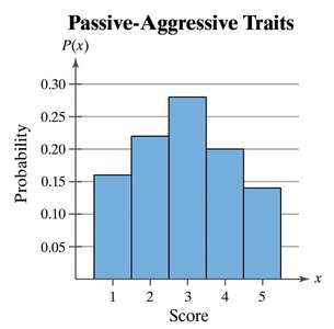
Graph: The histogram visually represents the probability distribution, showing symmetry and the distribution of scores.

Identifying Valid Probability Distributions

To determine if a distribution is valid, check:

• Each probability is between 0 and 1.

• The sum of all probabilities equals 1.

Example: If the sum is greater than 1 or any probability is negative, the distribution is not valid.

Mean of a Discrete Probability Distribution

The mean (expected value) of a discrete probability distribution is calculated by multiplying each value by its probability and summing the results.

• Formula: $\mu = \sum xP(x)$

• Example: For the personality inventory test, $\mu = 1 \times 0.16 + 2 \times 0.22 + 3 \times 0.28 + 4 \times 0.20 + 5 \times 0.14 = 2.94$

• Interpretation: The mean score is slightly less than 3, indicating a tendency toward passive traits.

Variance and Standard Deviation of a Discrete Probability Distribution

Variance measures the spread of the distribution, while standard deviation is the square root of variance.

• Variance Formula: $\sigma^2 = \sum (x - \mu)^2 P(x)$

• Standard Deviation Formula: $\sigma = \sqrt{\sigma^2}$

Example: For the personality inventory test:

x	P(x)	x - μ	(x - μ)2	(x - μ)2P(x)
1	0.16	-1.94	3.764	0.602
2	0.22	-0.94	0.884	0.194
3	0.28	0.06	0.004	0.001
4	0.20	1.06	1.124	0.225
5	0.14	2.06	4.244	0.594

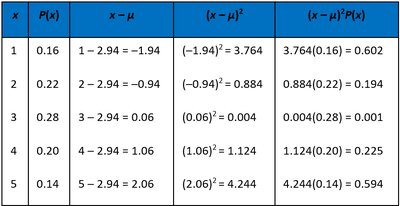
• Variance: $\sigma^2 = 1.6164$

• Standard Deviation: $\sigma = \sqrt{1.6164} \approx 1.27$

• Interpretation: Most scores differ from the mean by no more than 1.3.

Summary Table: Key Properties of Discrete Probability Distributions

Property	Description
Discrete Random Variable	Countable outcomes (e.g., number of sales calls)
Continuous Random Variable	Uncountable outcomes (e.g., hours spent)
Probability Distribution	List of values and their probabilities
Mean ($\mu$)	Expected value, $\mu = \sum xP(x)$
Variance ($\sigma^2$)	Spread, $\sigma^2 = \sum (x - \mu)^2 P(x)$
Standard Deviation ($\sigma$)	Square root of variance, $\sigma = \sqrt{\sigma^2}$