Displaying and Summarizing Data: Categorical and Quantitative Variables

Displaying and Summarizing Data

Introduction

In statistics, it is essential to summarize and display data effectively to reveal patterns, trends, and insights. The methods used depend on whether the variable is categorical or quantitative. This chapter covers the main techniques for visualizing and summarizing both types of variables, including tables, charts, and numerical summaries.

Summarizing and Displaying a Categorical Variable

Types of Univariate Categorical Displays

• Frequency and Relative Frequency Tables

• Bar Chart

• Pareto Chart

• Pie Chart

• Ring (Donut) Chart

Frequency Tables

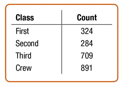
A frequency table lists each category and the number of observations in each category. This is a foundational tool for summarizing categorical data.

Class	Count
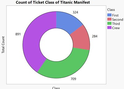
First	324
Second	284
Third	709
Crew	891

Relative Frequency Tables

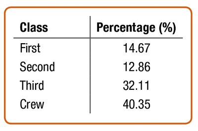
A relative frequency table shows the percentage of observations in each category, making it easier to compare groups of different sizes.

Class	Percentage (%)
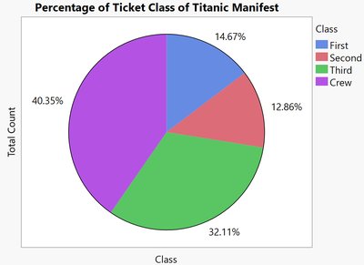
First	14.67
Second	12.86
Third	32.11
Crew	40.35

Bar Charts

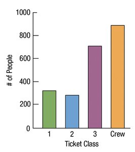
A bar chart displays the frequency or relative frequency of each category using bars of equal width. Bar charts are effective for comparing the sizes of different categories.

Pie Charts

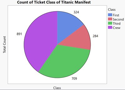
A pie chart represents each category as a slice of a circle, with the size of each slice proportional to the category's frequency or percentage. Pie charts are useful for showing the composition of a whole.

Ring (Donut) Charts

A ring chart (or donut chart) is similar to a pie chart but with a blank center. It also displays proportions of categories as segments of a ring.

Pareto Charts

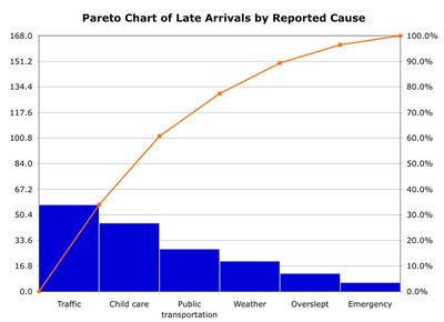
A Pareto chart is a bar chart with categories ordered from most to least frequent. It often includes a line showing cumulative frequency or percentage, highlighting the most significant categories.

Displaying a Quantitative Variable

Types of Univariate Quantitative Displays

• Histograms

• Stem-and-Leaf Plots

• Dotplots

Histograms

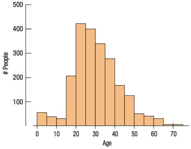
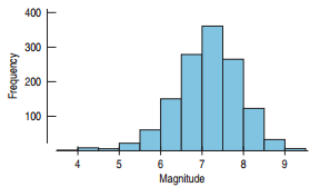
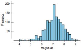
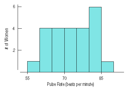
A histogram displays the distribution of a quantitative variable by grouping data into bins of equal width. The height of each bar shows the number of observations within each bin.

Effect of Bin Width

The choice of bin width can affect the appearance and interpretation of a histogram. Narrow bins show more detail, while wider bins provide a broader overview.

Stem-and-Leaf Displays

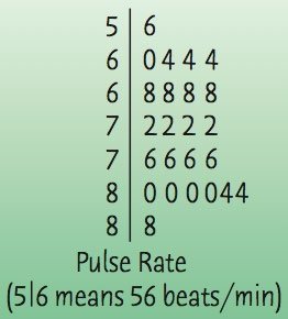
A stem-and-leaf plot shows the distribution of a quantitative variable while preserving individual data values. It is best for small data sets and resembles a vertical histogram.

Dotplots

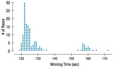
A dotplot uses dots to represent individual data points, showing the shape of the distribution. Dotplots are useful for small data sets.

Describing a Distribution

Shape, Center, and Spread

When describing a distribution, always address three aspects:

• Shape: The overall form of the distribution (e.g., symmetric, skewed, unimodal, bimodal).

• Center: The typical or central value (e.g., mean, median).

• Spread: The variability or dispersion of the data (e.g., range, interquartile range, standard deviation).

Shape of the Distribution

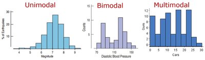
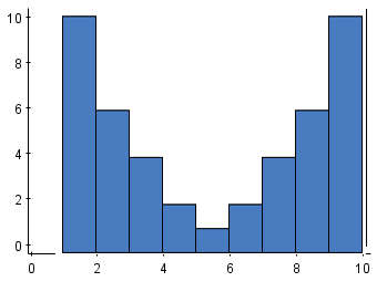
• Modes: Peaks in the histogram are called modes. One peak is unimodal, two peaks are bimodal, and more than two are multimodal.

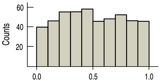
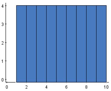
• Uniform: A histogram with roughly equal frequencies across bins is called uniform.

Symmetry and Skewness

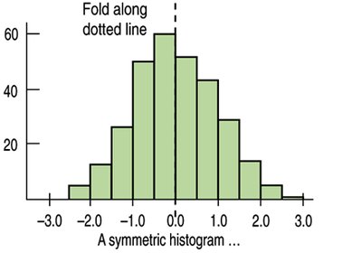
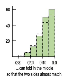
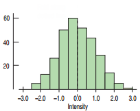
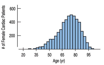
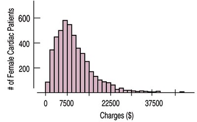
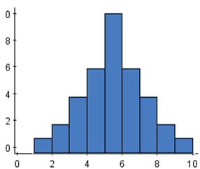
A distribution is symmetric if it can be folded along a vertical line through the center so that both sides match. If one tail is longer, the distribution is skewed in the direction of the longer tail.

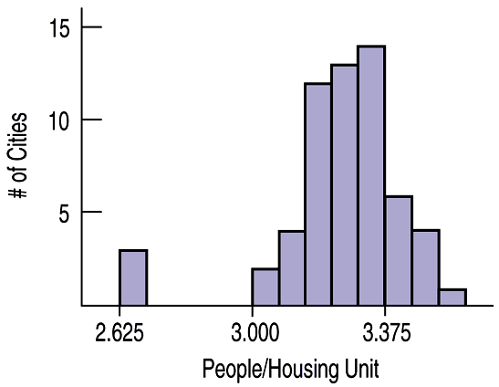
Unusual Features

Look for outliers (values far from the rest) and gaps (empty bins), which may indicate special causes or subgroups in the data.

Center of a Distribution

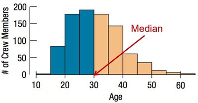
Median

The median is the value with half the data below and half above. It is resistant to outliers and is preferred for skewed distributions.

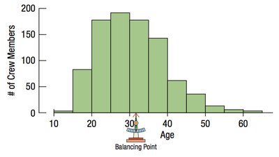
Mean

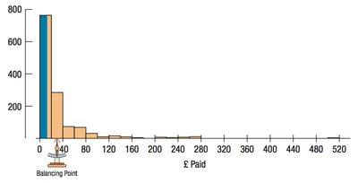
The mean (arithmetic average) is the sum of all values divided by the number of values. It is sensitive to outliers and is best used for symmetric distributions without outliers.

Formula for the mean:

$\bar{y} = \frac{\sum y}{n}$

Spread of a Distribution

Range

The range is the difference between the maximum and minimum values. It is sensitive to extreme values and may not represent the overall spread well.

Percentiles and Quartiles

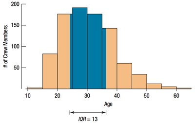
Percentiles divide the data into 100 equal parts. The quartiles divide the data into four equal parts: Q1 (25th percentile), Q2 (median, 50th percentile), and Q3 (75th percentile).

Interquartile Range (IQR)

The interquartile range (IQR) is the difference between the upper and lower quartiles (Q3 - Q1). It measures the spread of the middle 50% of the data and is resistant to outliers.

$\mathrm{IQR} = Q_3 - Q_1$

Standard Deviation and Variance

The standard deviation (s) measures the average distance of data values from the mean. The variance (s2) is the average squared deviation from the mean.

Variance formula:

$s^2 = \frac{\sum (y - \bar{y})^2}{n-1}$

Standard deviation formula:

$s = \sqrt{\frac{\sum (y - \bar{y})^2}{n-1}}$

Interpreting Standard Deviation

A small standard deviation means data are tightly clustered around the mean; a large standard deviation means data are more spread out.

Comparing Spread with Histograms

Histograms with more spread out bars have larger standard deviations. Comparing histograms visually can help estimate which has greater variability.

Summary: What to Tell About Variables

• For categorical variables: Use frequency/relative frequency tables, bar charts, pie charts, or ring charts. Report counts or percentages.

• For quantitative variables: Use histograms, stem-and-leaf plots, or dotplots. Describe shape, center, and spread. Use median and IQR for skewed data; mean and standard deviation for symmetric data.

• Always note any unusual features, such as outliers or multiple modes.