Dynamic Causal Effects and Distributed Lag Models in Time Series Econometrics

Dynamic Causal Effects in Time Series

Introduction to Dynamic Causal Effects

Dynamic causal effects describe how a change in an independent variable (X) affects a dependent variable (Y) over time. In economics and statistics, understanding these effects is crucial for policy analysis and forecasting. For example, the effect of a freeze in Florida on orange juice prices may persist for several months, not just immediately.

• Definition: The effect on Y of a change in X over time, measured at various future points.

• Examples: The effect of a change in the Federal Funds rate on inflation over several months; the effect of a tax increase on cigarette consumption over several years.

The Orange Juice Data Example

Data Description

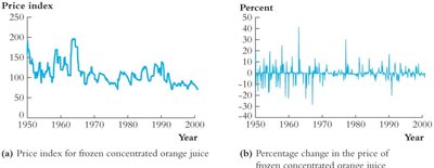
The orange juice data set is used to illustrate dynamic causal effects. It includes monthly data from January 1950 to December 2000 (T = 612):

• FDD (Freezing Degree Days): Number of days in a month with temperatures below 32°F, weighted by degrees below freezing.

• Price: Price index for frozen concentrated orange juice.

• %ChgP: Percentage change in price at an annual rate, calculated as $1200 \Delta \ln(Price_t)$.

Distributed Lag Model

Model Specification

The distributed lag (DL) model estimates the effect of current and past values of X on Y. It is particularly useful in time series when the effect of X is not immediate but distributed over several periods.

• General Form:

$Y_t = \beta_0 + \beta_1 X_t + \beta_2 X_{t-1} + \cdots + \beta_{r+1} X_{t-r} + u_t$

• Impact Effect (\(\beta_1\)): Immediate effect of X on Y.

• Dynamic Multipliers (\(\beta_2, \beta_3, \ldots\)): Effects of lagged values of X on Y.

• Cumulative Dynamic Multiplier: Sum of the impact and lagged effects up to a certain period.

Assumptions of the Distributed Lag Model

• 1. Exogeneity: $E(u_t | X_t, X_{t-1}, X_{t-2}, \ldots) = 0$

• 2. Stationarity: Y and X have stationary distributions; as lag increases, observations become independent.

• 3. Finite Moments: Y and X have eight nonzero finite moments (important for HAC standard errors).

• 4. No Perfect Multicollinearity: The regressors are not perfectly collinear.

Estimation and Standard Errors

Heteroskedasticity and Autocorrelation Consistent (HAC) Standard Errors

In time series, errors may be both heteroskedastic and autocorrelated. Standard OLS errors are inconsistent in this context. HAC standard errors, such as the Newey-West estimator, adjust for these issues.

• Variance Formula:

$\text{var}(\hat{\beta}_1) = \frac{1}{T} \frac{\sigma_v^2}{(\sigma_X^2)^2} \times f_T$

• Newey-West Estimator: $\hat{f}_T = 1 + 2 \sum_{j=1}^{m-1} \frac{m-j}{m} \hat{\rho}_j$

• Truncation Parameter (m): Rule of thumb: $m = 0.75 \times T^{1/3}$

Cumulative Multipliers and Their Standard Errors

Computation and Interpretation

Cumulative multipliers measure the total effect of a one-time change in X over several periods. They are calculated by summing the distributed lag coefficients. Their standard errors are computed as linear combinations of the estimated coefficients, using HAC standard errors.

• Example (with 1 lag):

$Y_t = \beta_0 + \beta_1 X_t + \beta_2 X_{t-1} + u_t$

Can be rewritten as:

$Y_t = \beta_0 + \beta_1 \Delta X_t + (\beta_1 + \beta_2) X_{t-1} + u_t$

• Impact Effect: $\delta_1 = \beta_1$

• First Cumulative Multiplier: $\delta_2 = \beta_1 + \beta_2$

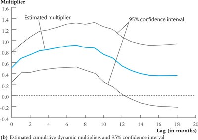
Table: Dynamic and Cumulative Multipliers

The following table summarizes estimated dynamic and cumulative multipliers for the effect of a freezing degree day (FDD) on orange juice prices (selected lags):

Lag Number	Dynamic Multipliers	Cumulative Multipliers
0	0.50 (0.14)	0.50 (0.14)
1	0.17 (0.09)	0.67 (0.14)
2	0.07 (0.06)	0.74 (0.17)
3	0.07 (0.04)	0.81 (0.18)
4	0.02 (0.03)	0.84 (0.19)
5	0.03 (0.03)	0.87 (0.19)
18	0.00 (0.02)	0.37 (0.30)

Graphical Representation

The estimated cumulative dynamic multipliers and their 95% confidence intervals show that the effect of a freeze on orange juice prices peaks several months after the event and then gradually declines.

Testing Stability of Dynamic Effects

QLR Statistic and Structural Breaks

Stability of the estimated dynamic effects can be tested using the Quandt Likelihood Ratio (QLR) statistic, which detects structural breaks in time series regression coefficients. Critical values depend on the number of restrictions and the trimming percentage.

• Interpretation: If the QLR statistic exceeds the critical value, there is evidence of a structural break in the relationship.

Summary Table: QLR Critical Values (Selected)

Number of Restrictions (q)	10%	5%	1%
1	7.12	8.68	12.16
5	3.26	3.66	4.53
10	2.48	2.71	3.23
15	2.16	2.34	2.71

Conclusion

Dynamic causal effects and distributed lag models are essential tools in time series econometrics for understanding how shocks propagate over time. Proper estimation requires attention to exogeneity, stationarity, and robust standard errors. The orange juice example illustrates these concepts in practice, including the importance of testing for structural breaks and interpreting cumulative effects.