Essential Study Guide for Introductory Statistics: Key Concepts, Definitions, and Applications

Chapter 1: Introduction to Statistics

Key Definitions and Concepts

This chapter introduces foundational terminology and concepts in statistics, focusing on the distinction between populations and samples, types of data, and study designs.

• Population vs. Sample: A population is the entire group of individuals or items of interest, while a sample is a subset of the population used for analysis.

• Parameter vs. Statistic: A parameter is a numerical summary of a population; a statistic is a numerical summary of a sample.

• Statistical vs. Practical Significance: Statistical significance means a result is unlikely to have occurred by chance, while practical significance considers whether the result is meaningful in real-world terms.

• Pitfalls in Data Analysis: Common issues include misleading conclusions and voluntary response bias.

• Quantitative vs. Categorical Data: Quantitative data are numerical and measurable; categorical data represent categories or groups.

• Levels of Measurement: Data can be nominal (categories), ordinal (ordered categories), interval (ordered, meaningful differences, no true zero), or ratio (ordered, meaningful differences, true zero).

• Observational Study vs. Experiment: Observational studies observe subjects without intervention; experiments involve manipulation of variables.

• Sampling Methods: Convenience (easy to reach), systematic (every nth item), stratified (subgroups sampled), cluster (groups sampled entirely).

• Types of Observational Studies: Cross-sectional, retrospective, and prospective.

• Blind vs. Double-Blind Experiments: Blind means subjects do not know treatment; double-blind means both subjects and experimenters are unaware.

Frequency Distributions and Histograms

Understanding how to read and construct frequency distributions and histograms is essential for visualizing data and inferring distribution shapes.

• Frequency Distribution: A table showing how data are distributed across categories or intervals.

• Histogram: A bar graph representing the frequency distribution of quantitative data; bars touch to indicate continuous data.

• Distribution Shape: Can be symmetric, skewed left/right, or uniform.

Chapter 2: Exploring Data with Tables and Graphs

Visual Displays and Their Interpretation

This chapter focuses on identifying and interpreting various visual displays of data, as well as recognizing misleading graphs.

• Types of Visual Displays: Histogram (quantitative), bar chart (categorical), time-series (data over time), scatterplot (relationship between two variables).

• Misleading Visual Displays: Graphs can mislead by manipulating axes, omitting baselines, or distorting proportions.

• Correlation: Scatterplots show correlation; r (correlation coefficient) quantifies strength and direction.

• Properties of r: $-1 \leq r \leq 1$; positive r indicates positive correlation, negative r indicates negative correlation; values near 0 suggest weak or no correlation.

• Correlation vs. Causation: Correlation does not imply causation.

Example: Identifying Misleading Graphs

Consider the following bar chart:

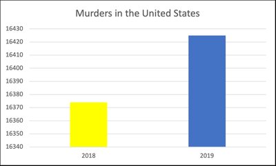
• Issue: The y-axis does not start at zero, exaggerating the difference between the two years.

• Explanation: When the y-axis is truncated, small differences appear much larger, misleading viewers about the magnitude of change.

Chapter 3: Describing, Exploring, and Comparing Data

Measures of Center and Variability

This chapter covers how to summarize data using measures of center and spread, and how to identify outliers.

• Measures of Center: Mean (average), median (middle value), mode (most frequent), midrange (average of max and min).

• Measures of Variance: Range (max - min), standard deviation (spread from mean), variance (average squared deviation).

• Resistant vs. Non-Resistant Measures: Median is resistant to outliers; mean is not.

• Range Rule of Thumb: Values more than 2 standard deviations from the mean are considered significant.

• Empirical Rule: For bell-shaped distributions: 68% within 1 SD, 95% within 2 SD, 99.7% within 3 SD.

• Z-Score: $z = \frac{x - \text{mean}}{\text{standard deviation}}$; compares values across different data sets.

• Five-Number Summary: Minimum, Q1, Median, Q3, Maximum.

• Boxplot: Visualizes five-number summary; helps identify outliers.

• IQR Rule for Outliers: $\text{IQR} = Q_3 - Q_1$; outliers are values below $Q_1 - 1.5 \times \text{IQR}$ or above $Q_3 + 1.5 \times \text{IQR}$.

Example: Calculating Z-Score

• Given: Mean = 952.22, St. Dev = 154.59, Value = 901

• Calculation: $z = \frac{901 - 952.22}{154.59} = -0.33$

Example: Identifying Outliers Using IQR

• Given: Q1 = 7, Q3 = 68

• Calculation: $\text{IQR} = 68 - 7 = 61$

• Lower Bound: $7 - 1.5 \times 61 = -84.5$

• Upper Bound: $68 + 1.5 \times 61 = 159.5$

• Conclusion: No values outside these bounds; no outliers.

Chapter 4: Probability

Basic Probability Concepts and Calculations

This chapter introduces probability, sample spaces, and calculation methods, including the use of tables and rules for combining events.

• Sample Space: The set of all possible outcomes of a procedure.

• Relative Frequency Approach: $P(A) = \frac{\text{number of times A occurs}}{\text{total number of trials}}$

• Classical Approach: $P(A) = \frac{\text{number of favorable outcomes}}{\text{number of possible outcomes}}$

• Interpreting Probability: Probability quantifies the likelihood of an event in context.

• Using Tables: Probabilities can be computed from tabular data.

• Addition Rule: For disjoint events: $P(A \text{ or } B) = P(A) + P(B)$

• Multiplication Rule: For independent events: $P(A \text{ and } B) = P(A) \times P(B)$

• Disjoint Events: Events that cannot occur together; $P(A \text{ and } B) = 0$

• Independent Events: Occurrence of one does not affect the other.

Example: Probability from a Table

Consider the following table summarizing candy preferences by team:

	Chocolate	Sour Candy	Total
Red	31	18	49
Blue	21	29	50
Yellow	26	23	49
Total	78	70	148

• Probability a student prefers chocolate: $P = \frac{78}{148}$

• Conditional Probability: $P(B|A)$ is the probability a student prefers chocolate given they are on the blue team.

• Disjoint Events: Blue team and chocolate preference are not disjoint; students can belong to both categories.

Example: Probability with Dice

• Probability Alex rolls a prime number: $P = \frac{3}{6} = 0.5$ (primes: 2, 3, 5)

• Probability Bella rolls odd then factor of 8: $P = \frac{9}{36} = 0.25$ (odd: 1, 3, 5; factors of 8: 1, 2, 4)

Example: Addition Rule for Disjoint Events

• Given: $P(A) = 0.26$, $P(B) = 0.20$; A and B are disjoint.

• Calculation: $P(A \text{ or } B) = 0.26 + 0.20 = 0.46$

Chapter Review: Key Terms and Symbols

Word Bank Applications

• Disjoint: Two events A and B are disjoint if $P(A \text{ and } B) = 0$

• Sample Variance: Notation is $s^2$

• Nominal Level: Most categorical level of measurement