Estimating a Population Mean and Determining Sample Size: Confidence Intervals and the Student t Distribution

Estimating a Population Mean

Introduction to Confidence Intervals

The main goal of this section is to present methods for using a sample mean \( \bar{x} \) to make an inference about the value of the corresponding population mean \( \mu \). Confidence intervals provide a range of plausible values for the population mean based on sample data, along with a specified level of confidence.

Key Concepts and Notation

• Population Mean (\( \mu \)): The average value in the entire population.

• Sample Mean (\( \bar{x} \)): The average value in the sample.

• Margin of Error (E): The maximum expected difference between the sample mean and the true population mean.

• Sample Size (n): The number of observations in the sample.

• Sample Standard Deviation (s): The measure of variability in the sample.

Constructing a Confidence Interval for the Population Mean

Requirements for Estimating \( \mu \) with Unknown \( \sigma \)

To construct a confidence interval for the population mean when the population standard deviation \( \sigma \) is unknown, the following requirements must be met:

• The sample is a simple random sample.

• The population is normally distributed, or the sample size is greater than 30 (n > 30).

Student t Distribution

When \( \sigma \) is unknown, the Student t distribution is used. The t distribution is similar to the standard normal distribution but has greater variability, especially for small sample sizes. The number of degrees of freedom is df = n - 1.

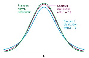
• The t distribution is symmetric and bell-shaped.

• Mean of t distribution is 0.

• Standard deviation is greater than 1 and decreases as sample size increases.

• As n increases, the t distribution approaches the standard normal distribution.

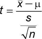
Formula for the t Statistic

The t statistic is calculated as:

$t = \frac{\bar{x} - \mu}{s / \sqrt{n}}$

Critical Value \( t_{\alpha/2} \)

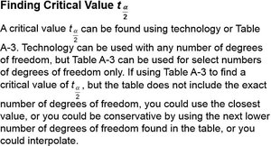
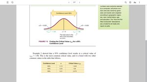
The critical value \( t_{\alpha/2} \) separates an area of \( \alpha/2 \) in the right tail of the Student t distribution. It is used to determine the margin of error for the confidence interval.

Finding the Critical Value \( t_{\alpha/2} \)

To find \( t_{\alpha/2} \), use technology (such as Excel) or a t distribution table. If the exact degrees of freedom are not listed, use the closest value or interpolate.

Procedure for Constructing a Confidence Interval

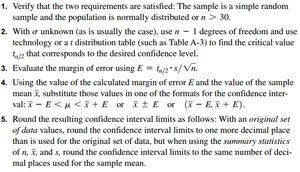
Follow these steps to construct a confidence interval for \( \mu \) when \( \sigma \) is unknown:

1. Verify requirements: simple random sample and normal population or n > 30.

2. Find the critical value \( t_{\alpha/2} \) for df = n - 1.

3. Calculate margin of error: $E = t_{\alpha/2} \cdot \frac{s}{\sqrt{n}}$

4. Construct the confidence interval: $\bar{x} - E < \mu < \bar{x} + E$

5. Round confidence interval limits appropriately.

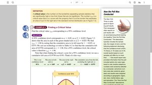
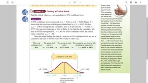
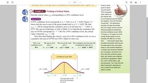
Example: Finding a Critical Value

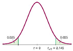
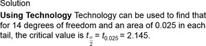
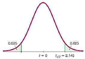
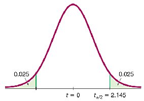
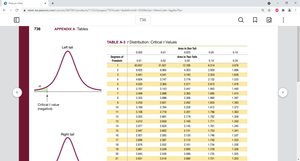
Find the critical value \( t_{\alpha/2} \) for a 95% confidence level with n = 15:

• Degrees of freedom: df = 15 - 1 = 14

• Area in each tail: 0.025

• Critical value: $t_{0.025} = 2.145$

Using Excel for Confidence Intervals

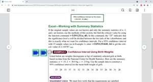
Excel can be used to calculate confidence intervals using the function =CONFIDENCE.T(alpha, standard_dev, size).

Determining Sample Size for Estimating \( \mu \)

Sample Size Formula

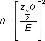
To estimate the value of a population mean with a specified margin of error, use the following formula:

$n = \left[ \frac{z_{\alpha/2} \cdot \sigma}{E} \right]^2$

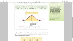
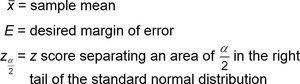
• \( z_{\alpha/2} \): z score for desired confidence level

• \( \sigma \): population standard deviation

• \( E \): desired margin of error

If the computed sample size is not a whole number, round up to the next whole number.

Dealing with Unknown \( \sigma \)

• Estimate \( \sigma \) using the range rule of thumb: \( \sigma \approx \text{range}/4 \)

• Use sample standard deviation \( s \) from preliminary data.

• Use results from previous studies.

Example: IQ Scores of Statistics Students

Suppose we want to estimate the mean IQ score for statistics students with 95% confidence and a margin of error of 3 IQ points. Assume \( \sigma = 15 \).

$n = \left[ \frac{1.96 \cdot 15}{3} \right]^2 = 96.04 \approx 97$

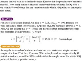
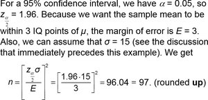
Interpretation: With a simple random sample of 97 students, we are 95% confident that the sample mean is within 3 IQ points of the true population mean.

Estimating \( \mu \) When \( \sigma \) Is Known

Confidence Interval Formula with Known \( \sigma \)

When the population standard deviation \( \sigma \) is known, use the standard normal distribution (z distribution) for the confidence interval:

$E = z_{\alpha/2} \cdot \frac{\sigma}{\sqrt{n}}$

$\bar{x} - E < \mu < \bar{x} + E$

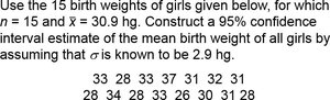
Example: Birth Weights of Girls

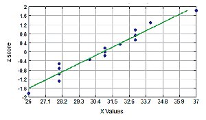
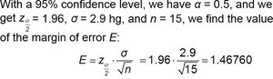
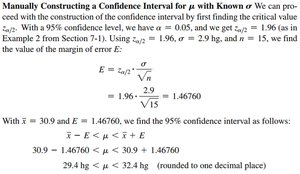
Given n = 15, \( \bar{x} = 30.9 \) hg, \( \sigma = 2.9 \) hg, construct a 95% confidence interval:

• \( z_{\alpha/2} = 1.96 \)

• Margin of error: $E = 1.96 \cdot \frac{2.9}{\sqrt{15}} = 1.46760$

• Confidence interval: $30.9 - 1.46760 < \mu < 30.9 + 1.46760$

• Result: $29.4 < \mu < 32.4$ hg (rounded to one decimal place)

Choosing Between t and z Distributions

When to Use Each Distribution

• Use the Student t distribution when \( \sigma \) is unknown and the sample size is small (n < 30).

• Use the z (normal) distribution when \( \sigma \) is known or the sample size is large (n > 30).

Summary Table: Confidence Interval Formulas

Situation	Distribution	Margin of Error Formula
\( \sigma \) unknown, n < 30	Student t	$E = t_{\alpha/2} \cdot \frac{s}{\sqrt{n}}$
\( \sigma \) known, any n	Standard normal (z)	$E = z_{\alpha/2} \cdot \frac{\sigma}{\sqrt{n}}$
\( \sigma \) unknown, n > 30	Student t (approximates z)	$E = t_{\alpha/2} \cdot \frac{s}{\sqrt{n}}$

Interpretation of Confidence Intervals

A confidence interval gives a range of values that, with a specified level of confidence (such as 95%), is likely to contain the true population mean. If many samples are taken, about 95% of the confidence intervals constructed will contain the true mean.

Additional info: The notes include practical examples, Excel functions, and step-by-step procedures for constructing confidence intervals and determining sample size, making them highly relevant for exam preparation in introductory statistics.