Estimating a Population Mean: Confidence Intervals and the t-Distribution

Estimating a Population Mean

Introduction to Confidence Intervals for the Mean

Estimating the population mean (μ) is a fundamental task in inferential statistics. Confidence intervals provide a range of plausible values for the population mean based on sample data. The method used depends on whether the population standard deviation (σ) is known or unknown.

Estimating a Mean When σ is Known

Confidence Interval Formula (σ Known)

When the population standard deviation is known (a rare scenario in practice), the confidence interval for the mean is constructed using the normal (z) distribution. The formula for the margin of error (E) is:

• Margin of Error (E): $E = z_{\alpha/2} \frac{\sigma}{\sqrt{n}}$

• Confidence Interval: $\bar{x} \pm E$

Where $z_{\alpha/2}$ is the critical value from the standard normal distribution for the desired confidence level, $\sigma$ is the population standard deviation, $n$ is the sample size, and $\bar{x}$ is the sample mean.

Sample Size for Estimating Mean (σ Known)

To achieve a desired margin of error, the required sample size can be calculated as:

$n = \left[ \frac{z_{\alpha/2} \sigma}{E} \right]^2$

Where $E$ is the desired margin of error.

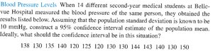
Example: Blood Pressure Levels

Suppose 14 medical students measured the blood pressure of the same person, and the population standard deviation is known to be 10 mmHg. The sample data and summary statistics are as follows:

Estimating a Mean When σ is Unknown (Most Common Case)

Using the t-Distribution

In practice, the population standard deviation (σ) is rarely known. Instead, the sample standard deviation (s) is used, introducing additional uncertainty. The confidence interval is then constructed using the t-distribution:

• Margin of Error (E): $E = t_{\alpha/2} \frac{s}{\sqrt{n}}$

• Confidence Interval: $\bar{x} \pm E$

Where $t_{\alpha/2}$ is the critical value from the t-distribution with $n-1$ degrees of freedom.

Properties of the t-Distribution

• Symmetric about mean = 0

• Wider than the z-distribution (greater variability, especially for small n)

• Shape depends on sample size (degrees of freedom, df = n - 1)

• As n increases, the t-distribution approaches the normal distribution

Historical Note: The Student's t-Distribution

The t-distribution was introduced by Sir William Gosset, who published under the pseudonym "Student" while working at the Guinness Brewery. His work highlighted the need for a larger critical value to account for the extra uncertainty when σ is unknown.

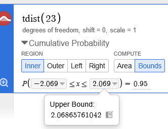
Finding the t Critical Value

The t critical value depends on the desired confidence level and the degrees of freedom. For example, for a 95% confidence interval with 23 degrees of freedom, the critical value is approximately 2.069.

Requirements for t-Intervals

To use the t-interval for estimating a mean, the following requirements must be met:

• The sample is a simple random sample (all samples of the same size have an equal chance of being selected).

• The value of the population standard deviation is unknown.

• Either the population is normally distributed, or the sample size is large (n > 30), or the sample data do not show strong departures from normality.

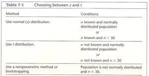
Choosing Between z and t

The following table summarizes when to use the z or t distribution, or a nonparametric method:

Method	Conditions
Use normal (z) distribution	σ known and normally distributed population or σ known and n > 30
Use t distribution	σ not known and normally distributed population or σ not known and n > 30
Use a nonparametric method or bootstrapping	Population is not normally distributed and n ≤ 30

Worked Example: Three-Minute Hourglass Timer

Constructing a 95% Confidence Interval

Suppose you measure the time for a three-minute hourglass and want to construct a 95% confidence interval for the average time. The process involves:

1. Calculating the sample mean and standard deviation from repeated measurements.

2. Determining the appropriate t critical value for the sample size.

3. Computing the margin of error and constructing the interval.

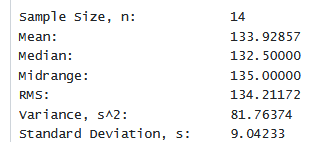
Summary Table: Descriptive Statistics Example

Descriptive statistics such as mean, standard deviation, skewness, and kurtosis are often calculated as part of the estimation process. These values help assess the distribution and suitability of the data for confidence interval estimation.

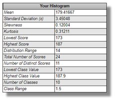
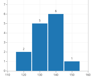
Visualizing Data: Histogram

Histograms are useful for visualizing the distribution of sample data, which is important for checking the normality assumption required for t-intervals.

Key Takeaways

• Use the z-interval when σ is known and the population is normal or n is large.

• Use the t-interval when σ is unknown and the population is normal or n is large.

• Check normality before applying t-intervals, especially for small samples.

• Sample size calculations are essential for achieving desired precision in estimates.