7.2 Estimating Population Means and Determining Sample Sizes: Confidence Intervals and the Student t Distribution

Estimating Parameters and Determining Sample Sizes

Estimating a Population Mean

Estimating the population mean is a fundamental task in statistics, especially when the population standard deviation (σ) is unknown. This section focuses on constructing confidence intervals for the population mean using sample data, and determining the sample size required for reliable estimation.

Confidence Interval for Estimating a Population Mean with σ Not Known

• Definition: A confidence interval is a range of values, derived from sample statistics, that is likely to contain the population mean (μ).

• Requirements:

  • The sample must be a simple random sample.

  • The population should be normally distributed, or the sample size should be greater than 30 (n > 30).

  • If n < 30, assess normality: distribution should be symmetric, have no outliers, and only one mode.

• Margin of Error (E): The margin of error quantifies the uncertainty in the estimate of the population mean.

Confidence Interval Formula (σ Not Known)

When σ is unknown, the confidence interval is constructed using the Student t distribution:

$\bar{x} \pm t_{\alpha/2} \left( \frac{s}{\sqrt{n}} \right)$

• \bar{x}: Sample mean

• s: Sample standard deviation

• n: Sample size

• t_{\alpha/2}: Critical value from the t distribution with df = n - 1

Margin of Error Formula

$E = t_{\alpha/2} \left( \frac{s}{\sqrt{n}} \right)$

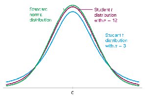
The Student t Distribution

The Student t distribution is used when the population standard deviation is unknown and the sample size is small. It is similar to the normal distribution but has heavier tails, which accounts for the increased variability in small samples.

• Origin: Developed by William Gosset ("Student") at Guinness Brewery for quality control experiments.

• Degrees of Freedom (df): The number of independent values in a sample that can vary. For confidence intervals, df = n - 1.

• Properties: The shape of the t distribution depends on the sample size; as n increases, it approaches the normal distribution.

Example of Degrees of Freedom: If you have 10 test scores with a fixed mean, 9 scores can vary freely, but the 10th is determined by the restriction, so df = 9.

Procedure for Constructing a Confidence Interval for μ

1. Verify requirements: random sample, normality or large sample size.

2. Calculate the sample mean (\bar{x}) and sample standard deviation (s).

3. Determine the degrees of freedom (df = n - 1).

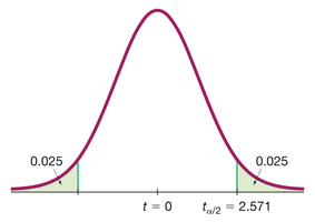
4. Find the critical value t_{\alpha/2} for the desired confidence level.

5. Compute the margin of error (E).

6. Construct the confidence interval: \bar{x} ± E.

Example: Confidence Interval Using Peanut Butter Cups

Suppose we have the following sample weights (grams) of Reese’s Peanut Butter Cups Miniatures: 8.639, 8.689, 8.548, 8.980, 8.936, 9.042. The package label states the total weight is 340.2 g for 38 cups, so the expected mean is 8.953 g.

• Point Estimate: Calculate the sample mean from the data.

• Constructing the Confidence Interval: Use the sample mean, sample standard deviation, and t distribution to find the interval.

• Normality Check: A normal quantile plot shows the data fits a straight-line pattern, indicating normality.

• Statistical Software: Technology (e.g., StatCrunch) can automate calculations and display the confidence interval limits.

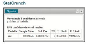
Result: The 95% confidence interval is 8.5901 g < μ < 9.0213 g. Since the expected mean (8.953 g) is within this interval, the package appears to be filled correctly.

Finding a Point Estimate and Margin of Error from a Confidence Interval

• Point Estimate: The sample mean (\bar{x}) is the best estimate of the population mean.

• Margin of Error: The margin of error (E) is half the width of the confidence interval.

Estimating a Population Mean When σ Is Known

If the population standard deviation (σ) is known, the confidence interval is constructed using the standard normal (z) distribution:

$\bar{x} \pm z_{\alpha/2} \left( \frac{\sigma}{\sqrt{n}} \right)$

• z_{\alpha/2}: Critical value from the standard normal distribution.

Choosing the Correct Distribution

• Use the t distribution when σ is unknown.

• Use the z distribution when σ is known.

Finding the Sample Size Required to Estimate a Population Mean

To ensure the sample mean is within a specified margin of error (E) of the population mean, calculate the required sample size:

$n = \left( \frac{z_{\alpha/2} \cdot \sigma}{E} \right)^2$

• Requirement: The sample must be a simple random sample.

• Round-Off Rule: If n is not a whole number, round up to the next integer.

Dealing with Unknown σ When Finding Sample Size

• Range Rule of Thumb: Estimate σ as range/4.

• Start and Improve: Begin with an estimated σ, refine as more data are collected.

• Use Prior Results: Use σ from previous studies or similar populations. Always err on the side of a larger sample size for reliability.

Example: IQ Scores of Statistics Students

Suppose we want to estimate the mean IQ score for statistics students, using a standard deviation of 15 (from Wechsler IQ tests). To be 95% confident that the sample mean is within 3 IQ points of the population mean, calculate the required sample size:

$n = \left( \frac{z_{0.025} \cdot 15}{3} \right)^2$

Round up the result to the next whole number.

Summary Table: Comparison of t and z Distributions

Distribution	When Used	Critical Value	Formula
Student t	σ unknown, n small	t_{\alpha/2}, df = n-1	$\bar{x} \pm t_{\alpha/2} \left( \frac{s}{\sqrt{n}} \right)$
Standard Normal (z)	σ known	z_{\alpha/2}	$\bar{x} \pm z_{\alpha/2} \left( \frac{\sigma}{\sqrt{n}} \right)$