Chapter 9: Estimating the Value of a Parameter: Confidence Intervals for Proportions, Means, and Variances

Study Guide - Smart Notes

Tailored notes based on your materials, expanded with key definitions, examples, and context.

Estimating the Value of a Parameter

Estimating a Population Proportion

Estimating a population proportion involves using sample data to infer the value of a population parameter. The main tools are point estimates and confidence intervals.

Point Estimate: The value of a statistic that estimates the value of a parameter. For a population proportion, the point estimate is \( \hat{p} = \frac{x}{n} \), where x is the number of individuals with the characteristic and n is the sample size.
Confidence Interval: An interval of numbers based on a point estimate, designed to capture the true parameter with a specified level of confidence.

Example: In a survey of 2019 adults, 1252 frequently worry about their financial situation. The sample proportion is \( \hat{p} = \frac{1252}{2019} \approx 0.620 \).

Constructing and Interpreting Confidence Intervals for a Population Proportion

A confidence interval for a population proportion is constructed using the sampling distribution of \( \hat{p} \). For large enough samples, this distribution is approximately normal.

Mean of \( \hat{p} \): \( \mu_{\hat{p}} = p \)
Standard Error: \( \sigma_{\hat{p}} = \sqrt{\frac{p(1-p)}{n}} \)
95% Confidence Interval: \( \hat{p} \pm 1.96 \sigma_{\hat{p}} \)

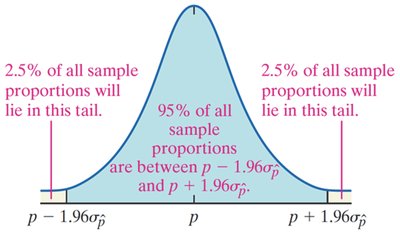
Normal distribution showing 95% of sample proportions within 1.96 standard errors of p

The margin of error determines the width of the interval. For a 95% confidence interval, 95% of all sample proportions will result in intervals containing the population proportion, while 5% will not.

General (1 – α)·100% Confidence Interval: \( \hat{p} \pm z_{\alpha/2} \sigma_{\hat{p}} \)

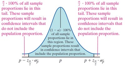
General confidence interval for a population proportion with alpha tails

The value \( z_{\alpha/2} \) is the critical value from the standard normal distribution for the desired confidence level.

Level of Confidence	Area in Each Tail	Critical Value (\( z_{\alpha/2} \))
90%	0.05	1.645
95%	0.025	1.96
99%	0.005	2.575

Interpretation: A (1 – α)·100% confidence interval means that (1 – α)·100% of all such intervals from repeated samples will contain the true parameter.

Determining Sample Size for Estimating a Proportion

To estimate a population proportion within a specified margin of error E, solve for n:

\( n = \left( \frac{z_{\alpha/2}}{E} \right)^2 \hat{p}(1-\hat{p}) \)
If no prior estimate, use \( \hat{p} = 0.5 \) for maximum variability.

Estimating a Population Mean

When estimating a population mean, the sample mean \( \bar{x} \) is used as the point estimate. Confidence intervals are constructed using the t-distribution when the population standard deviation is unknown.

Student’s t-Distribution: Used when \( \sigma \) is unknown and the sample is from a normal population or n is large.
t-Statistic: \( t = \frac{\bar{x} - \mu}{s/\sqrt{n}} \), where s is the sample standard deviation.

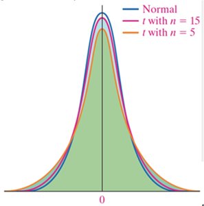
Comparison of normal and t-distributions for different sample sizes

The t-distribution is wider with heavier tails for smaller n, approaching the normal distribution as n increases.

Constructing and Interpreting Confidence Intervals for a Population Mean

(1 – α)·100% Confidence Interval: \( \bar{x} \pm t_{\alpha/2,\,df} \frac{s}{\sqrt{n}} \), where df = n – 1.
Check normality for small samples (n < 30) using normal probability plots or boxplots.

Determining Sample Size for Estimating a Mean

\( n = \left( \frac{z_{\alpha/2} s}{E} \right)^2 \), rounded up to the next integer.

Choosing the Appropriate Confidence Interval

To determine which confidence interval to use, consider the parameter of interest and the data conditions.

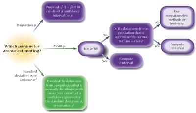
Flowchart for choosing the appropriate confidence interval method

For proportions, use the normal approximation if conditions are met.
For means, use the t-distribution if the population is normal or n is large.
For variances or standard deviations, use the chi-square distribution if the population is normal.

Estimating a Population Standard Deviation or Variance

To estimate the population variance (\( \sigma^2 \)) or standard deviation (\( \sigma \)), use the chi-square distribution. The sample variance (\( s^2 \)) is the point estimate.

The chi-square distribution is not symmetric and depends on degrees of freedom (df = n – 1).

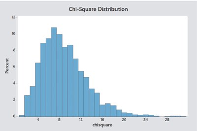
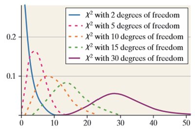
Histogram of chi-square distribution Chi-square distributions for different degrees of freedom

As degrees of freedom increase, the distribution becomes more symmetric.

Degrees of Freedom	Shape
Low (e.g., 2, 5)	Highly skewed right
High (e.g., 30)	Nearly symmetric

Confidence Interval for \( \sigma^2 \):

Lower bound: \( \frac{(n-1)s^2}{\chi^2_{\alpha/2}} \) Upper bound: \( \frac{(n-1)s^2}{\chi^2_{1-\alpha/2}} \)

To find a confidence interval for \( \sigma \), take the square root of the bounds above.

Estimating with Bootstrapping

Bootstrapping is a nonparametric, computer-intensive method for estimating parameters and constructing confidence intervals when parametric assumptions are not met.

Resample the observed data with replacement many times (e.g., 1000 or 10,000 resamples).
Calculate the statistic of interest for each resample.
Use the distribution of these statistics to estimate confidence intervals (e.g., using percentiles).

Requirements: The bootstrap distribution should be centered near the original sample statistic and be symmetric.

Summary Table: Confidence Interval Methods

Parameter	Point Estimate	Interval Method	Distribution
Proportion (p)	\( \hat{p} \)	\( \hat{p} \pm z_{\alpha/2} \sqrt{\frac{\hat{p}(1-\hat{p})}{n}} \)	Normal
Mean (\( \mu \))	\( \bar{x} \)	\( \bar{x} \pm t_{\alpha/2,\,df} \frac{s}{\sqrt{n}} \)	t-distribution
Variance (\( \sigma^2 \))	\( s^2 \)	See above	Chi-square