Examining Residuals and the Residual Standard Deviation in Linear Regression

Linear Regression: Examining Residuals

Introduction to Residuals in Regression

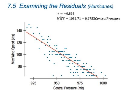
In linear regression, residuals are the differences between observed values and the values predicted by the regression model. Examining residuals is crucial for assessing the appropriateness of a regression model and for diagnosing potential problems with the fit.

• Residual (e): The difference between the observed value (Y) and the predicted value (\( \hat{Y} \)), calculated as \( e = Y - \hat{Y} \).

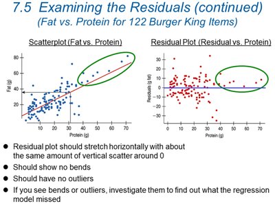
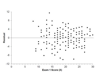
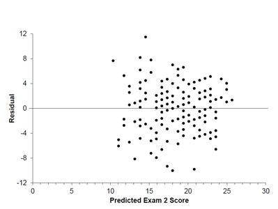
• After fitting a regression model, we plot the residuals to check for patterns. Ideally, the residual plot should show no systematic structure.

• A scatterplot of residuals versus the x-values (or versus predicted values) should appear random, with no clear direction, shape, or outliers.

Purpose of Residual Plots

Residual plots help us determine whether the regression model adequately captures the relationship between variables. They are used to check for:

• Non-linearity (bends or curves in the plot)

• Outliers (points far from the rest)

• Non-constant variance (spread of residuals changes across values of x)

Key Points:

• The residual plot should stretch horizontally with about the same amount of vertical scatter around zero.

• There should be no bends or outliers. If present, investigate further as the regression model may be missing important features.

Understanding the Residual Standard Deviation (\( S_e \))

Definition and Calculation

The residual standard deviation (also called the standard error of estimate) measures the typical vertical distance of the data points from the regression line. It quantifies the average prediction error made by the regression model.

• Formula:

$S_e = \sqrt{\frac{\sum (Y - \hat{Y})^2}{n - 2}} = \sqrt{\frac{\sum e^2}{n - 2}}$

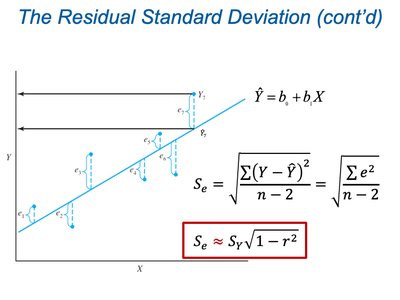
• Alternatively, when summary statistics are available, use:

$S_e \approx S_Y \sqrt{1 - r^2}$

• Where \( S_Y \) is the standard deviation of Y, and r is the correlation coefficient.

Interpreting \( S_e \)

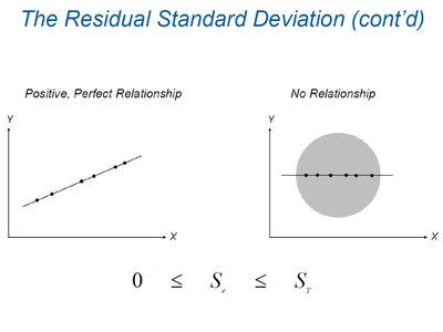
\( S_e \) tells us, on average, how much the observed values deviate from the regression line. The smaller the \( S_e \), the better the model fits the data.

• For a perfect linear relationship (r = 1), \( S_e = 0 \).

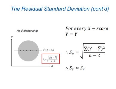
• For no relationship (r = 0), \( S_e \approx S_Y \).

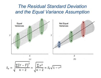
Equal Variance Assumption (Homoscedasticity)

Definition and Importance

The equal variance assumption (homoscedasticity) states that the variability of the residuals should be roughly constant across all values of the explanatory variable (x). This is a key condition for valid inference in regression analysis.

• If the scatter diagram is elliptical (football-shaped) and there are no outliers, the equal variance assumption likely holds.

• If the spread of residuals increases or decreases with x, the assumption is violated (heteroscedasticity).

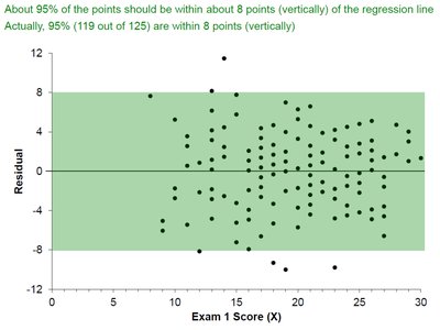
Empirical Rule for Residuals

If the equal variance assumption holds, the distribution of residuals follows a pattern similar to the empirical rule for normal distributions:

• About 68% of points are within one \( S_e \) of the regression line (vertically).

• About 95% are within two \( S_e \).

• About 99.7% are within three \( S_e \).

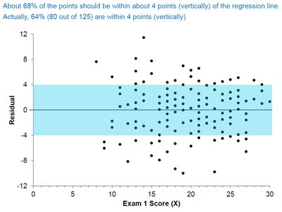
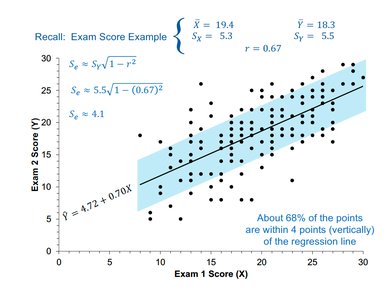
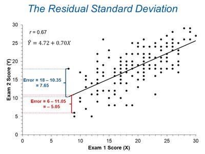
Worked Example: Exam Scores

Regression and Residuals

Consider a regression model predicting Exam 2 scores (Y) from Exam 1 scores (X):

$\hat{Y} = 4.72 + 0.70X$

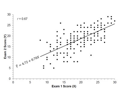
• The residuals are the vertical distances from each point to the regression line.

Calculating \( S_e \) for the Example

• Given: \( S_Y = 5.5 \), \( r = 0.67 \)

• \( S_e \approx 5.5 \sqrt{1 - (0.67)^2} = 4.1 \)

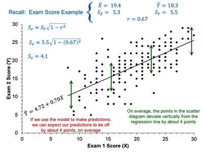
On average, predictions deviate from the regression line by about 4 points.

Visualizing the Empirical Rule with Residuals

• About 68% of the points are within 4 points (vertically) of the regression line.

• About 95% are within 8 points, and 99.7% are within 12 points.

Summary Table: Residual Standard Deviation Formulas

Situation	Formula for \( S_e \)	Interpretation
General case	$S_e = \sqrt{\frac{\sum (Y - \hat{Y})^2}{n - 2}}$	Standard deviation of residuals
Using summary statistics	$S_e \approx S_Y \sqrt{1 - r^2}$	Approximate, especially for large n
Perfect relationship (r = 1)	$S_e = 0$	No prediction error
No relationship (r = 0)	$S_e \approx S_Y$	All variation remains unexplained

Application: Using Software Output

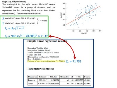
Statistical software often reports the residual standard deviation (sometimes labeled as "s" or "Std Error of Estimate") in regression output. For example, in a regression predicting Math SAT scores from Verbal SAT scores:

• \( S_e \) is reported as 71.755

• Alternatively, calculate using summary statistics: \( S_e \approx 98.1 \sqrt{1 - (0.685)^2} = 71.47 \)

Key Takeaways

• Residuals and their standard deviation are essential for diagnosing regression models.

• Residual plots should show no pattern; patterns indicate model inadequacy.

• The residual standard deviation quantifies the typical prediction error.

• The equal variance assumption must be checked for valid inference.

• Use summary statistics or software output to compute \( S_e \).