Exploring Data with Tables and Graphs: Frequency Distributions and Comparative Analysis

Describing Data with Tables and Graphs

Frequency Distributions for Organizing and Summarizing Data

Frequency distributions are essential tools in statistics for organizing and summarizing large data sets. They help reveal the underlying patterns and distribution of the data, making it easier to interpret and analyze.

• Frequency Distribution (or Frequency Table): Shows how data are partitioned among several categories (or classes) by listing the categories along with the number (frequency) of data values in each.

• Purpose: To organize raw data into a more comprehensible format, highlighting the distribution and frequency of values.

Key Terms in Frequency Distributions

• Lower Class Limits: The smallest numbers that can belong to each of the different classes.

• Upper Class Limits: The largest numbers that can belong to each of the different classes.

• Class Boundaries: The numbers used to separate the classes, eliminating gaps between class intervals.

• Class Width: The difference between two consecutive lower class limits in a frequency distribution. Formula: $\text{Class Width} = \text{(Maximum Value - Minimum Value)} \div \text{Number of Classes}$

• Class Midpoints: The values in the middle of the classes, calculated as: $\text{Class Midpoint} = \frac{\text{Lower Class Limit} + \text{Upper Class Limit}}{2}$

Procedure for Constructing a Frequency Distribution

1. Select the number of classes (usually between 5 and 20).

2. Calculate the class width and round up to a convenient number.

3. Choose the first lower class limit (often the minimum value or a convenient value below it).

4. List the lower class limits, adding the class width successively.

5. Determine the upper class limits for each class.

6. Tally each data value into the appropriate class and count the frequencies.

Example: McDonald’s Lunch Service Times

The following data set represents drive-through service times (in seconds) for McDonald’s lunches:

Following the procedure, the frequency distribution is constructed as follows:

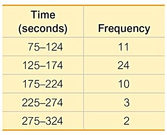
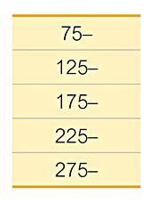
Lower class limits are listed vertically to help identify corresponding upper class limits:

The final frequency table summarizes the data:

Relative Frequency and Cumulative Frequency Distributions

• Relative Frequency Distribution: Each class frequency is replaced by a relative frequency (proportion) or a percentage. Formula: $\text{Relative Frequency} = \frac{\text{Class Frequency}}{\text{Sum of All Frequencies}}$

• Percentage Frequency: The relative frequency expressed as a percentage. Formula: $\text{Percentage Frequency} = \text{Relative Frequency} \times 100\%$

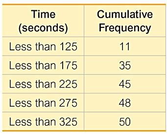
• Cumulative Frequency Distribution: The frequency for each class is the sum of the frequencies for that class and all previous classes.

Example of a cumulative frequency distribution for McDonald’s lunch service times:

Interpreting Frequency Distributions

• Normal Distribution: Frequencies start low, increase to a maximum, and then decrease, forming a roughly symmetric pattern.

• Gaps: The presence of gaps in a frequency distribution can indicate data from two or more different populations.

Example: Exploring Data with Gaps

The following table shows the frequency distribution of the weights of randomly selected pennies:

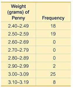
A large gap between the lightest and heaviest pennies suggests two populations: pennies made after 1983 (mostly zinc) and those made before 1983 (mostly copper).

Comparing Data Sets Using Relative Frequency Distributions

Combining two or more relative frequency distributions in one table facilitates comparison between data sets.

Example: Comparing McDonald’s and Dunkin’ Donuts Service Times

The table below compares the relative frequency distributions for drive-through lunch service times at McDonald’s and Dunkin’ Donuts:

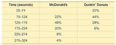
By comparing the relative frequencies, it is evident that Dunkin’ Donuts generally has lower service times than McDonald’s.