Exploring Data with Tables and Graphs: Introductory Statistics Study Notes

Exploring Data with Tables and Graphs

Frequency Distributions for Organizing and Summarizing Data

Frequency distributions are essential tools in statistics for organizing and summarizing large data sets. They help reveal the nature of the distribution and facilitate further analysis.

• Frequency Distribution: A table that shows how data are partitioned among several categories (or classes) by listing the categories along with the number (frequency) of data values in each.

• Relative Frequency: The proportion of data values in each category, calculated as the frequency divided by the total number of data values.

• Percentage Distribution: The percentage of data values in each category, calculated as the relative frequency multiplied by 100.

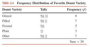
• Example: Favorite donut varieties among 30 people.

Formula for Percentage:

$\text{Percentage} = (\text{Relative frequency}) \times 100\%$

Constructing Frequency Distributions

To construct a frequency distribution for quantitative data, follow these steps:

• Select the number of classes (usually between 5 and 20).

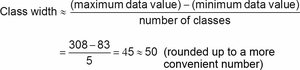
• Calculate the class width using the formula:

$\text{Class width} \approx \frac{\text{maximum data value} - \text{minimum data value}}{\text{number of classes}}$

• Choose the first lower class limit (often the minimum value or a convenient value below it).

• List the lower and upper class limits for each class.

• Assign each data value to a class and tally the frequencies.

Histograms

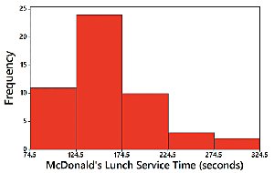
A histogram is a graphical representation of a frequency distribution for quantitative data. Bars of equal width are drawn adjacent to each other, with the height representing the frequency.

• Uses: Visualizes the shape, center, spread, and outliers of the data.

• Relative Frequency Histogram: Similar to a histogram, but the vertical axis shows relative frequencies.

• Example: McDonald's lunch service times.

Common Distribution Shapes

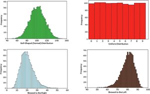
Histograms can reveal different shapes of distributions:

• Normal (Bell-Shaped) Distribution: Symmetric, with most values clustered around the center.

• Uniform Distribution: All values are equally likely.

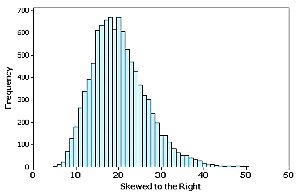
• Skewed Right: Longer tail on the right side.

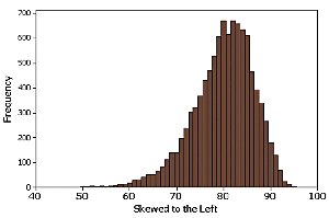
• Skewed Left: Longer tail on the left side.

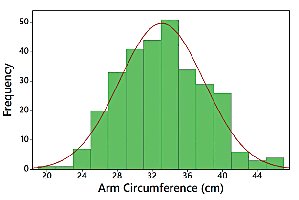
Normal Distribution

A normal distribution is characterized by its bell-shaped curve, indicating that data are symmetrically distributed around the mean.

Skewness

Skewness describes the asymmetry of a distribution:

• Right (Positive) Skew: The tail extends more to the right.

• Left (Negative) Skew: The tail extends more to the left.

Single-Valued Classes

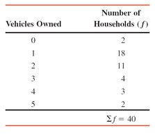
For discrete data with a small number of possible values, each value can be treated as a class in the frequency distribution.

• Example: Number of vehicles owned by households.

Pie Charts

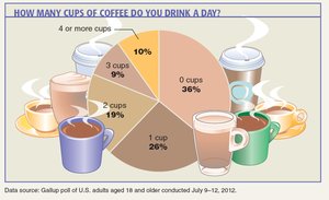
Pie charts display categorical data as slices of a circle, with each slice proportional to the frequency or percentage of the category.

• Example: Cups of coffee consumed per day.

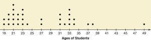
Dotplots

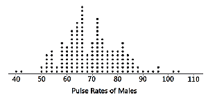
Dotplots are used for quantitative data, plotting each data value as a dot above a horizontal scale. Dots representing equal values are stacked.

• Features: Displays the shape of the distribution and allows reconstruction of the original data.

• Example: Pulse rates of males.

• Example: Ages of students in a statistics class.

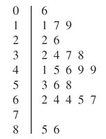
Stemplots (Stem-and-Leaf Plots)

Stemplots represent quantitative data by splitting each value into a stem and a leaf. They retain the original data values and show the shape of the distribution.

• Example: Pulse rates of males.

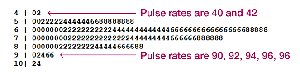
• Example: Grouped stem-and-leaf display for hours spent on computers.

Bar Graphs

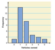
Bar graphs use bars of equal width to show frequencies of categories for categorical (qualitative) data. Bars may be separated by gaps.

• Feature: Facilitates comparison of different categories.

• Example: Vehicles owned by households.

Pareto Charts

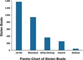
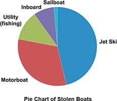
Pareto charts are bar graphs for categorical data, with bars arranged in descending order of frequency. They highlight the most important categories.

• Example: Stolen boats by type.

Pie Charts (Categorical Data)

Pie charts are commonly used to show the distribution of categorical data.

• Example: Stolen boats by type.

Frequency Polygons

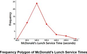
Frequency polygons use line segments connected to points above class midpoints to show the distribution of quantitative data. They are similar to histograms but use lines instead of bars.

• Relative Frequency Polygon: Uses relative frequencies for the vertical scale.

• Example: McDonald's lunch service times.

Cumulative Frequency Distributions

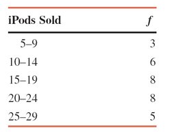
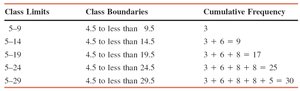
A cumulative frequency distribution shows the total number of values that fall below the upper boundary of each class.

• Example: Number of iPods sold by a company.

Cumulative Frequency Table:

Class Limits	Class Boundaries	Cumulative Frequency
5–9	4.5 to less than 9.5	3
5–14	4.5 to less than 14.5	9
5–19	4.5 to less than 19.5	17
5–24	4.5 to less than 24.5	25
5–29	4.5 to less than 29.5	30

Cumulative Relative Frequency and Cumulative Percentage

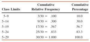
Cumulative relative frequency and cumulative percentage distributions show the proportion and percentage of values below each class boundary.

Class Limits	Cumulative Relative Frequency	Cumulative Percentage
5–9	3/30 = .100	10.0
5–14	9/30 = .300	30.0
5–19	17/30 = .567	56.7
5–24	25/30 = .833	83.3
5–29	30/30 = 1.000	100.0