Exploring Data with Tables and Graphs: Frequency Distributions and Graphical Summaries

Frequency Distributions

Constructing a Frequency Distribution

A frequency distribution (or frequency table) organizes data into categories (or classes) and shows the number of data values in each class. This is a foundational tool for summarizing large data sets and identifying patterns.

• Step 1: Select the number of classes (usually 5–20). The choice may depend on convenience and the range of data values.

• Step 2: Calculate the class width: $\text{Class width} \approx \frac{\text{Maximum data value} - \text{Minimum data value}}{\text{Number of classes}}$ Round up to a convenient number.

• Step 3: Choose the first lower class limit (often the minimum value or a convenient value below it).

• Step 4: List other lower class limits by adding the class width successively.

• Step 5: List lower class limits vertically, then determine and enter upper class limits.

• Step 6: Tally each data value into the appropriate class and sum tallies for class frequencies.

Classes should not overlap, and each value must belong to exactly one class. All classes should be included, even those with zero frequency. Consistent class width is preferred, though sometimes open-ended intervals are necessary.

Relative and Percentage Frequency Distributions

• Relative frequency: $\text{Relative frequency for a class} = \frac{\text{Frequency for a class}}{\text{Sum of all frequencies}}$

• Percentage frequency: $\text{Percentage for a class} = \frac{\text{Frequency for a class}}{\text{Sum of all frequencies}} \times 100\%$

• The sum of percentages should be close to 100% (allowing for rounding errors).

Normal and Non-Normal Distributions

• Normal distribution: Frequencies start low, increase to a peak, then decrease, forming a symmetric, bell-shaped curve.

• Non-normal distribution: May show skewness, gaps, or patterns indicating multiple populations.

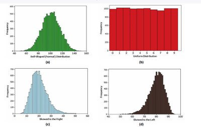
Distribution Shapes and Skewness

• Symmetric (Normal): Frequencies are mirrored around the center.

• Skewed Right (Positively Skewed): Longer right tail (e.g., income data).

• Skewed Left (Negatively Skewed): Longer left tail (e.g., human lifespan data).

Class Boundaries, Midpoints, and Cumulative Frequency

• Lower class limits: Smallest numbers in each class.

• Upper class limits: Largest numbers in each class.

• Class boundaries: Numbers separating classes without gaps.

• Class midpoints: $\text{Class midpoint} = \frac{\text{Lower class limit} + \text{Upper class limit}}{2}$

• Class width: Difference between consecutive lower class limits.

• Cumulative frequency: Each class frequency is the sum of its own and all previous class frequencies.

Graphical Summaries of Data

Histograms

A histogram is a bar graph for quantitative data, where the horizontal axis represents classes and the vertical axis represents frequencies. Bars are adjacent unless there are gaps in the data.

• Relative frequency histogram: Uses proportions or percentages on the vertical axis instead of raw frequencies.

• Histograms help visualize the distribution, center, and spread of data.

Normal Quantile Plots

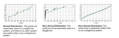
Normal quantile plots help assess whether data are approximately normally distributed.

• If points lie close to a straight line, the distribution is normal.

• Systematic deviations from a straight line indicate non-normality.

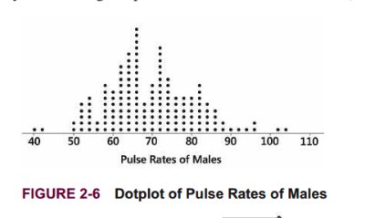
Dotplots

A dotplot displays each data value as a dot above a horizontal scale. Stacked dots represent repeated values. Dotplots reveal the shape of the distribution and allow for reconstruction of the original data set.

Stemplots (Stem-and-Leaf Plots)

A stemplot separates each value into a "stem" (e.g., leftmost digit) and a "leaf" (e.g., rightmost digit). Stemplots retain original data values and show the distribution's shape. Data are sorted in order.

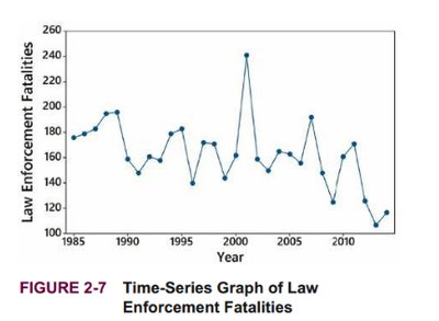
Time-Series Graphs

A time-series graph plots quantitative data collected at different points in time, revealing trends and patterns over time.

Bar Graphs

A bar graph uses bars of equal width to show frequencies of categories for categorical (qualitative) data. Bars may be separated by gaps. Bar graphs facilitate comparison of different categories.

Pareto Charts

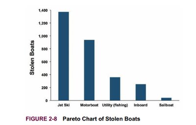
A Pareto chart is a bar graph for categorical data, with bars arranged in descending order of frequency. This highlights the most important categories.

Pie Charts

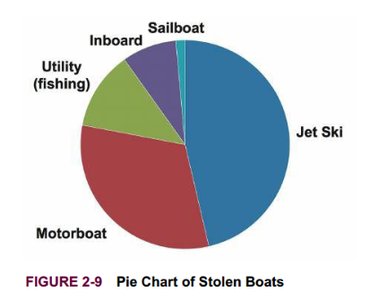
A pie chart depicts categorical data as slices of a circle, with each slice proportional to the category's frequency. Pie charts are common but less effective than Pareto charts for comparison.

Frequency Polygons

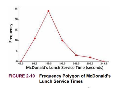
A frequency polygon uses line segments connected to points above class midpoints to display frequency distributions. Relative frequency polygons use proportions or percentages and allow for comparison of multiple data sets on one graph.

Misleading Graphs

• Vertical scales starting above zero can exaggerate differences.

• Pictographs (using images instead of bars) can distort data due to area or volume effects.

Scatterplots and Correlation

Scatterplots

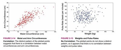
A scatterplot displays paired (x, y) quantitative data, with the x-axis for the first variable and the y-axis for the second. Scatterplots reveal relationships (correlation) between variables.

• Correlation: Exists when values of one variable are associated with values of another.

• Linear correlation: Points form a pattern approximated by a straight line.

• Correlation does not imply causation.

Regression Line

The regression line (line of best fit or least-squares line) is the straight line that best fits the scatterplot data, used for prediction and analysis.

Key Vocabulary

• Center: A value representing the middle of the data set.

• Variation: The amount by which data values differ.

• Distribution: The shape or spread of data values (e.g., bell-shaped).

• Outliers: Values far from the majority of data.

• Time: Changes in data characteristics over time.

Summary Table: Types of Graphs and Their Uses

Graph Type	Data Type	Main Purpose
Histogram	Quantitative	Show frequency distribution
Dotplot	Quantitative	Display distribution and original values
Stemplot	Quantitative	Show distribution and retain data
Time-Series Graph	Quantitative (over time)	Show trends over time
Bar Graph	Categorical	Compare category frequencies
Pareto Chart	Categorical	Highlight most frequent categories
Pie Chart	Categorical	Show proportion of categories
Frequency Polygon	Quantitative	Compare distributions
Scatterplot	Paired Quantitative	Show correlation between variables

Additional info: This summary integrates textbook-style explanations, formulas, and examples to provide a comprehensive overview of graphical data exploration in introductory statistics.