Frequency Distributions and Graphs in Introductory Statistics

Frequency Distributions and Graphs

Characteristics of Data

Understanding data involves examining several key characteristics that describe its overall structure and behavior:

• Center: The central value or typical value of a data set (e.g., mean, median, mode).

• Variation: The degree to which data values differ from each other (e.g., range, variance, standard deviation).

• Distribution: The overall shape and spread of the data values.

• Outliers: Data values that are significantly different from the majority of the data.

• Time: The sequence or timing of data collection, important for time-series data.

Frequency Distributions

A frequency distribution (or frequency table) organizes data into categories or classes, showing how many data values fall into each class. This helps summarize large data sets and reveals patterns in the data.

• Lower Class Limits: The smallest values that can belong to each class.

• Upper Class Limits: The largest values that can belong to each class.

• Class Boundaries: Values that separate classes without gaps, typically halfway between upper and lower class limits.

• Class Midpoints: The value in the middle of each class, calculated as (lower class limit + upper class limit) / 2.

• Class Width: The difference between consecutive lower class limits or boundaries.

Formula for Class Width:

$\text{Class Width} = \frac{\text{Maximum Value} - \text{Minimum Value}}{\text{Number of Classes}}$

Constructing a Frequency Distribution Table

To build a frequency distribution table, follow these steps:

1. Determine the number of classes (usually between 5 and 20).

2. Calculate the class width (round up if necessary).

3. Choose a starting point for the first lower class limit (often the minimum value).

4. List the lower class limits for each class.

5. Determine the upper class limits for each class.

6. Find the class boundaries.

7. Tally the data into classes and record the frequencies.

8. Calculate cumulative and relative frequencies as needed.

Relative Frequency: The proportion of data values in each class.

$\text{Relative Frequency} = \frac{\text{Class Frequency}}{\text{Sum of All Frequencies}}$

Percentage Frequency: The percentage of data values in each class.

$\text{Percentage Frequency} = \frac{\text{Class Frequency}}{\text{Sum of All Frequencies}} \times 100\%$

Histograms

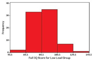
A histogram is a bar graph representing the frequency distribution of quantitative data. The horizontal axis shows the classes, and the vertical axis shows the frequencies. Bars are adjacent to each other, indicating continuous data.

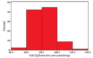
Relative Frequency Histogram: Similar to a histogram, but the vertical axis shows relative frequencies (proportions or percentages) instead of counts.

Interpreting Histograms and Distribution Shapes

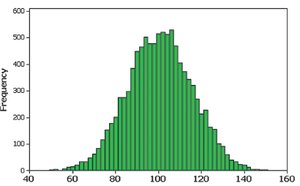
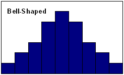
Histograms help identify the shape of the data distribution, the center, variation, and outliers. A normal distribution appears bell-shaped and symmetric.

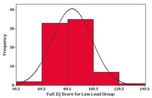
• Bell-shaped (Normal): Frequencies increase to a maximum at the center and decrease symmetrically.

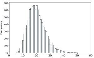
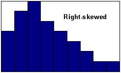
• Skewed Right (Positively Skewed): Longer right tail; most data are on the left.

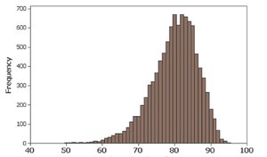
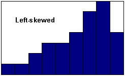
• Skewed Left (Negatively Skewed): Longer left tail; most data are on the right.

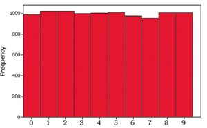
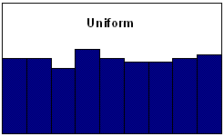
• Uniform: All classes have roughly the same frequency.

Common Distribution Shapes

• Bell-Shaped

• Uniform

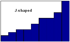
• J-Shaped

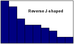
• Reverse J-Shaped

• Right-Skewed

• Left-Skewed

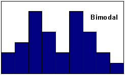
• Bimodal

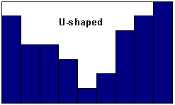
• U-Shaped

Assessing Normality

To determine if data are normally distributed, use:

• Histogram: Should be bell-shaped for normality.

• Outliers: Multiple outliers suggest non-normality.

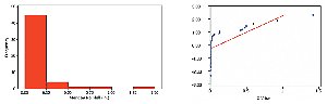
• Normal Quantile Plot: If points are close to a straight line, the data are likely normal.

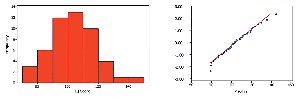
If the histogram is uniform or the quantile plot is not linear, the data are not normal.

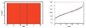
Skewed data will show a non-linear pattern in the quantile plot.

Frequency Polygons

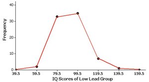
A frequency polygon uses line segments to connect points above class midpoints, showing the distribution's shape.

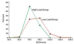
A relative frequency polygon uses proportions or percentages on the vertical axis.

Dotplots

A dotplot displays each data value as a dot above its value on a number line. Stacked dots indicate repeated values.

Stemplots (Stem-and-Leaf Plots)

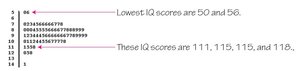
A stemplot separates each value into a stem (e.g., tens digit) and a leaf (e.g., units digit), preserving the original data values and showing distribution shape.

Scatterplots

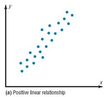
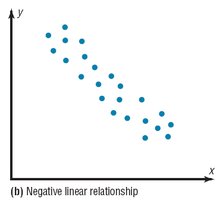
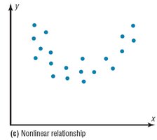
A scatterplot displays paired (x, y) data to reveal relationships between two quantitative variables.

• Positive Linear Relationship: Both variables increase together.

• Negative Linear Relationship: One variable increases as the other decreases.

• Nonlinear Relationship: The relationship follows a curve.

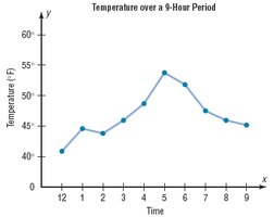
Time-Series Graphs

A time-series graph plots data collected at different points in time, showing trends or patterns over time.

Bar Graphs

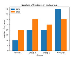
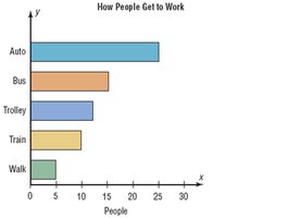
Bar graphs use bars of equal width to represent frequencies of categorical (qualitative) data. The vertical axis shows frequency or relative frequency, and the horizontal axis lists categories. Multiple bar graphs compare two or more data sets.

Pareto Charts

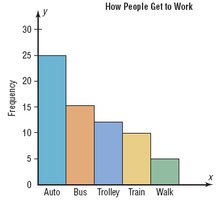
A Pareto chart is a bar graph for qualitative data, with bars arranged in descending order of frequency.

Pie Graphs

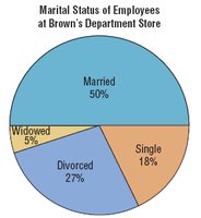
Pie graphs (or pie charts) show qualitative data as slices of a circle, with each slice proportional to the frequency count.

Misleading Graphs

Some graphs can be misleading due to errors or intentional distortion. Common issues include:

• Nonzero Axis: Starting an axis at a value other than zero exaggerates differences.

• Three-Dimensional Effects: Using 3D shapes for 1D data can distort perception of differences.

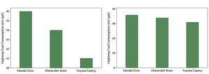
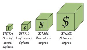
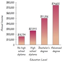
Example: A 3D bar for income may appear much larger than it should, misleading viewers about the actual difference in values.

Additional info: These notes cover the essential concepts of frequency distributions and graphical data representation, which are foundational for understanding and analyzing data in introductory statistics.