Fundamentals of Data Management and Statistics: Study Notes

Statistics: Foundations and Reasoning

What is Statistics?

Statistics is a systematic way of reasoning and thinking about data to uncover patterns and draw meaningful conclusions. It involves collecting, analyzing, and interpreting data to tell a story about the phenomena under study.

• Unit of Analysis (Who): The individual cases or subjects about which data are collected. Knowing "who" is essential for meaningful analysis.

• Variable (What): The characteristics recorded for each individual. Variables can be categorical, quantitative, or identifier variables.

• Data Collection: The method of data collection (planned experiment, survey, etc.) critically affects the validity of conclusions.

• The 5 Ws and H: Who, What, When, Where, Why, and How are key questions for statistical thinking.

Example: In a household income survey, "household" is the unit of analysis (who), and "income" is the variable (what).

Types of Variables

Categorical, Quantitative, and Identifier Variables

Variables are the recorded characteristics of each case. Understanding their types is crucial for proper analysis.

• Categorical (Qualitative) Variable: Names categories and answers questions about how cases fall into those categories (e.g., sex, race, ethnicity).

• Ordinal Variable: A ranking variable where the order matters but not the magnitude of difference (e.g., 1st, 2nd place).

• Quantitative Variable: Measured on a continuous scale, answers questions about the quantity (e.g., income, height, weight).

• Identifier Variable: Categorical variable with exactly one individual per category (e.g., SIN, ISBN). Not typically analyzed statistically.

Displaying and Summarizing Categorical Data

Visualizing Categorical Variables

Effective visualization is key to understanding and communicating data patterns. The area principle states that the area in a graph should reflect the magnitude of the value.

• Frequency Table: Records the totals for each category.

• Bar Chart: Displays counts for each category side by side for comparison. Relative frequency bar charts show proportions.

• Pie Chart: Shows parts of a whole, with each slice proportional to the category's fraction. Categories must be mutually exclusive.

Exploring Relationships Between Two Categorical Variables

• Contingency Table: Displays counts for combinations of two categorical variables. Margins show totals and marginal distributions.

• Conditional Distribution: Distribution of one variable for individuals satisfying a condition on another variable. Independence is indicated if distributions are the same across categories.

Displaying and Summarizing Quantitative Data

Histograms, Stem-and-Leaf, and Dotplots

Quantitative data are best visualized using histograms, stem-and-leaf displays, and dotplots. These methods reveal the distribution's shape, center, and spread.

• Histogram: Plots binned quantitative data. Bars touch unless a bin has no data. Shows distribution, not just comparison.

• Stem-and-Leaf Display: Preserves individual values while showing distribution. Stems label bins; leaves show data points.

• Dotplot: Places a dot for each case along an axis.

Describing Distributions

• Shape: Modality (number of peaks), symmetry, skewness, outliers.

• Center: Mode (most common value), median (middle value), mean (average).

• Spread: Range, interquartile range (IQR), variance, standard deviation.

Example: For a skewed distribution, use the median and IQR; for symmetric, use mean and standard deviation.

Measures of Spread

Range, IQR, Variance, and Standard Deviation

• Range: $\text{Range} = \text{Max} - \text{Min}$

• Interquartile Range (IQR): $\text{IQR} = Q_3 - Q_1$

• Variance: $s^2 = \frac{1}{n-1} \sum_{i=1}^n (x_i - \bar{x})^2$

• Standard Deviation: $s = \sqrt{s^2}$

Five Number Summary: Max, Q3, Median, Q1, Min.

Boxplots and Outliers

Constructing and Interpreting Boxplots

Boxplots graphically display the five-number summary and are useful for comparing groups. Outliers are shown as special symbols.

• Draw vertical axis, mark quartiles and median, connect to form box.

• Fences: 1.5 IQR above Q3 and below Q1 (not shown in final plot).

• Whiskers: Extend to most extreme values within fences.

• Outliers: Values beyond fences, marked with symbols.

The Standard Deviation as a Ruler and the Normal Model

Standardizing with Z-Scores

Standardizing values allows comparison across different scales. Z-scores measure the distance from the mean in standard deviations.

• Z-Score Formula: $z = \frac{x - \bar{x}}{s}$

• Shifting (adding/subtracting a constant) affects position, not spread.

• Scaling (multiplying/dividing by a constant) affects both position and spread.

Density Curves and the Normal Model

• Density Curve: Smooth curve modeling data distribution. Must be non-negative and total area = 1.

• Normal Model: $N(\mu, \sigma)$, where $\mu$ is mean and $\sigma$ is standard deviation (parameters).

• Standard Normal Model: $N(0,1)$

• 68-95-99.7 Rule: In a normal model, ~68% of values within 1 SD, ~95% within 2 SD, ~99.7% within 3 SD.

Normal Probability Plots

If data are roughly normal, the normal probability plot is a straight diagonal line. Deviations indicate non-normality.

Sampling and Surveys

Principles of Sampling

Sampling is used to draw conclusions about a population from a subset (sample). Proper sampling avoids bias and ensures representativeness.

• Examine a Part of the Whole: Use a sample to represent the population.

• Randomize: Random selection protects against bias.

• Sample Size: The size of the sample, not the population, determines representativeness.

Sampling Strategies

• Simple Random Sample (SRS): Every possible sample of the desired size has an equal chance of selection.

• Stratified Sampling: Population divided into homogeneous groups (strata); SRS taken within each stratum.

• Cluster Sampling: Population split into clusters; random clusters selected, census within clusters.

• Multistage Sampling: Combines several sampling methods.

• Systematic Sampling: Select every nth individual, starting from a random point.

Common Sampling Mistakes and Biases

• Voluntary Response Bias: Sample consists of volunteers, often unrepresentative.

• Convenience Sampling: Sample chosen for ease, not representativeness.

• Bad Sampling Frame: Incomplete list leads to bias.

• Undercoverage: Some population segments not sampled or underrepresented.

• Nonresponse Bias: Non-respondents may differ from respondents in key ways.

• Response Bias: Survey design influences responses (e.g., question wording, interviewer effects).

Parameters vs. Statistics

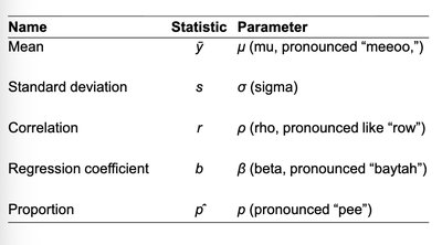
Parameters are key numbers in population models, denoted by Greek letters. Statistics are summaries from sample data, denoted by Latin letters.

Name	Statistic	Parameter
Mean	$\bar{y}$	$\mu$ (mu)
Standard deviation	$s$	$\sigma$ (sigma)
Correlation	$r$	$\rho$ (rho)
Regression coefficient	$b$	$\beta$ (beta)
Proportion	$\hat{p}$	$p$

Ensuring Valid Surveys

• Define what you want to know.

• Use the right sampling frame.

• Ask specific, quantitative questions.

• Pilot test your survey and report methods in detail.

Additional info: These notes cover foundational topics in statistics, including data types, visualization, measures of center and spread, the normal model, and sampling strategies. They are suitable for college-level statistics students preparing for exams or coursework.