 Back
BackHypothesis Testing: Concepts, Procedures, and Applications
Study Guide - Smart Notes
 Tailored notes based on your materials, expanded with key definitions, examples, and context.
Hypothesis Testing: Foundations and Procedures
The Language of Hypothesis Testing
Hypothesis testing is a fundamental inferential statistical procedure used to evaluate claims about population parameters based on sample data. It involves formulating two competing statements: the null hypothesis and the alternative hypothesis.
Null Hypothesis (H0): A statement of no effect, no difference, or status quo. It is assumed true until evidence suggests otherwise.
Alternative Hypothesis (H1 or Ha): The statement for which we seek supporting evidence. It represents a change, effect, or difference.
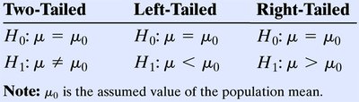
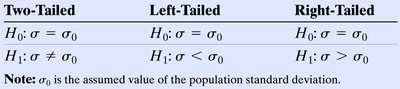
Hypotheses can be structured in three main ways, depending on the research question:
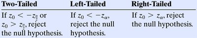
Two-tailed test: H0: parameter = value; H1: parameter ≠ value
Left-tailed test: H0: parameter = value; H1: parameter < value
Right-tailed test: H0: parameter = value; H1: parameter > value
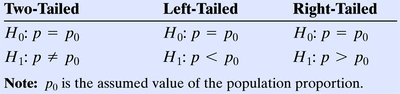
Additional info: The choice of test direction depends on the research hypothesis (e.g., 'different', 'less than', or 'greater than').
Errors in Hypothesis Testing: Type I and Type II
When making decisions based on sample data, two types of errors can occur:
Type I Error (α): Rejecting the null hypothesis when it is actually true. The probability of this error is denoted by α, the level of significance.
Type II Error (β): Failing to reject the null hypothesis when the alternative hypothesis is true. The probability of this error is denoted by β.
There is a trade-off between α and β: decreasing one typically increases the other.
Drawing Conclusions
After performing a hypothesis test, conclusions are stated in terms of rejecting or not rejecting the null hypothesis. We never "accept" the null hypothesis; instead, we say there is insufficient evidence to reject it.
Testing Hypotheses about a Population Proportion
Logic of Hypothesis Testing for Proportions
To test claims about a population proportion, we use the sampling distribution of the sample proportion (\( \hat{p} \)). If the sample size is large enough, the distribution of \( \hat{p} \) is approximately normal:
Mean: \( \mu_{\hat{p}} = p \)
Standard deviation: \( \sigma_{\hat{p}} = \sqrt{\frac{p(1-p)}{n}} \)
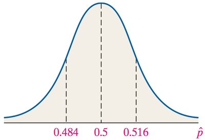
Statistical significance is determined by how unlikely the observed sample proportion is under the null hypothesis.
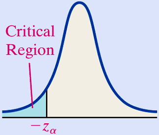
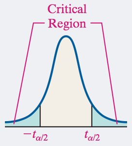
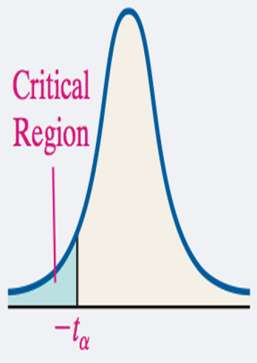
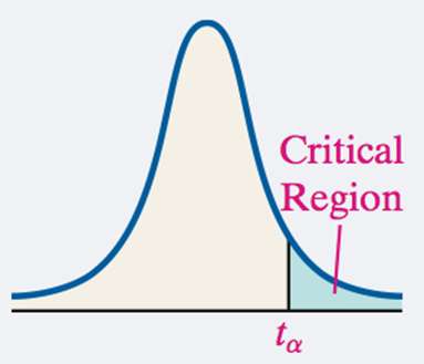
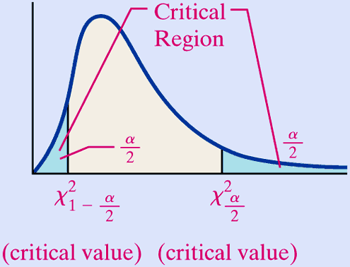
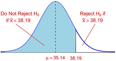
Classical Approach: Critical Value Method
We compare the test statistic to critical values to decide whether to reject H0. For a two-tailed test, the critical regions are in both tails of the normal distribution.
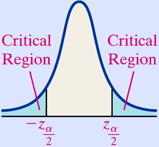
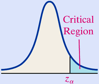
The test statistic for proportions is:
We reject H0 if the test statistic falls in the critical region.
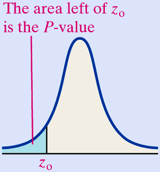
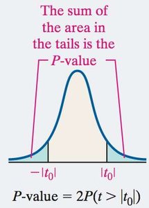
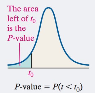
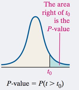
P-Value Approach
The P-value is the probability, under H0, of obtaining a result as extreme or more extreme than the observed sample statistic. For a two-tailed test, the P-value is the sum of the areas in both tails beyond the observed value.
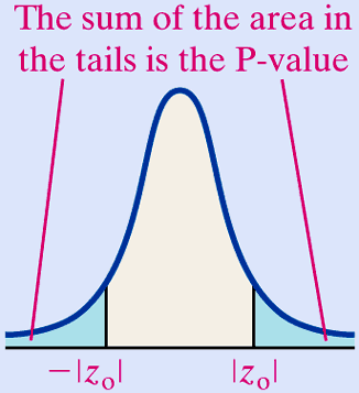
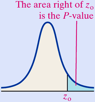
If the P-value is less than the significance level α, we reject H0.
Example: Large Sample Proportion Test
Suppose in a sample of 1010 adults, 525 do not trust the media. Test if the proportion has increased from 0.46 (1997) at α = 0.05.
H0: p = 0.46
H1: p > 0.46
Sample proportion: \( \hat{p} = 0.52 \)
Test statistic:
Critical value (right-tailed, α = 0.05): 1.645
Since 3.83 > 1.645, reject H0.
Conclusion: There is sufficient evidence to conclude the proportion has increased.
Small Sample Proportion Test: Binomial Approach
If the sample size is small and np(1-p) < 10, use the binomial probability distribution to compute the P-value directly.
Testing Hypotheses about a Population Mean
t-Distribution and Its Properties
When the population standard deviation is unknown, the t-distribution is used for hypothesis testing about means. The t-distribution:
Is symmetric and centered at 0
Has heavier tails than the normal distribution (more variability)
Approaches the normal distribution as sample size increases
Formulating Hypotheses for Means
Test Statistic for Means
The test statistic is:
where \( \bar{x} \) is the sample mean, \( \mu_0 \) is the hypothesized mean, s is the sample standard deviation, and n is the sample size.
Critical Value and P-Value Approaches
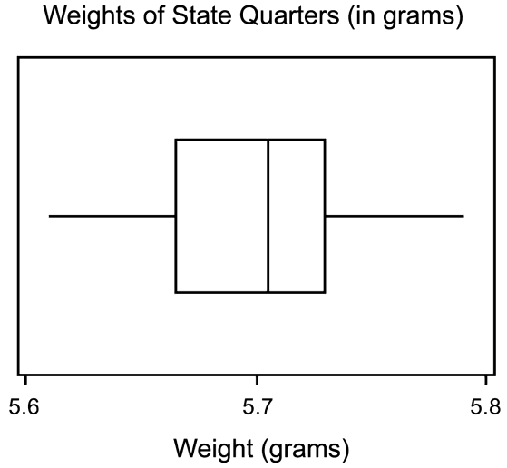
Example: Small Sample Mean Test
Suppose a researcher weighs 18 state quarters and finds a sample mean of 5.7022 grams (s = 0.0497). Test if the mean differs from 5.67 grams at α = 0.05.
H0: μ = 5.67
H1: μ ≠ 5.67
t0 = (5.7022 – 5.67) / (0.0497 / √18) = 2.75
Critical values (df = 17): ±2.11
Since 2.75 > 2.11, reject H0.
Conclusion: There is sufficient evidence to conclude the mean weight differs from 5.67 grams.
Statistical vs. Practical Significance
Statistical significance means the observed effect is unlikely under H0. Practical significance considers whether the effect size is large enough to be meaningful in context. Large samples can yield statistically significant but practically unimportant results.
Testing Hypotheses about a Population Standard Deviation
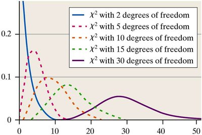
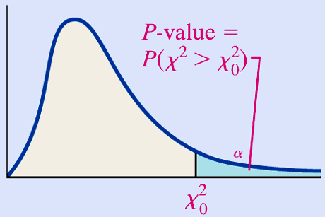
Chi-Square Distribution
The chi-square distribution is used to test hypotheses about population variance or standard deviation. It is not symmetric and depends on degrees of freedom (n – 1).
Formulating Hypotheses for Standard Deviation
Test Statistic for Variance/Standard Deviation
The test statistic is:
where s2 is the sample variance and σ02 is the hypothesized variance.
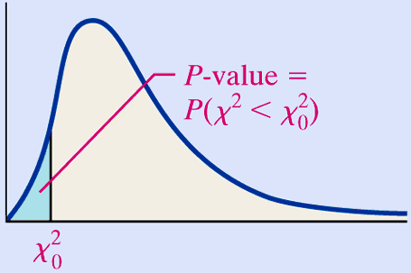
Critical Value and P-Value Approaches
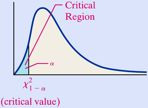
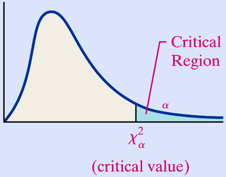
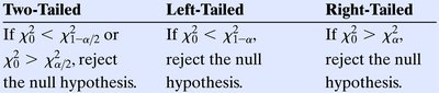
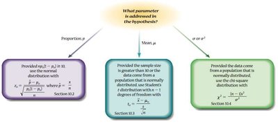
Choosing the Appropriate Hypothesis Test
The choice of test depends on the parameter of interest and the sample size:
Proportion (p): Use z-test if np(1-p) ≥ 10; otherwise, use binomial test.
Mean (μ): Use t-test if σ unknown and n > 30 or population is normal; use z-test if σ known.
Standard deviation (σ) or variance (σ2): Use chi-square test if population is normal.
Type II Error and Power of a Test
Probability of Type II Error (β)
Type II error occurs when we fail to reject H0 even though H1 is true. The probability β depends on the true value of the parameter, sample size, and significance level.
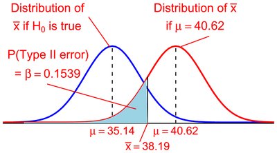
Power of a Test
The power of a test is the probability of correctly rejecting H0 when H1 is true. It is calculated as 1 – β. Higher power means a greater chance of detecting a true effect.
