 Back
BackHypothesis Testing for the Mean with the Student's t-Distribution (Small Samples)
Study Guide - Smart Notes
 Tailored notes based on your materials, expanded with key definitions, examples, and context.
Hypothesis Testing for the Mean with Small Samples
Introduction to Hypothesis Testing
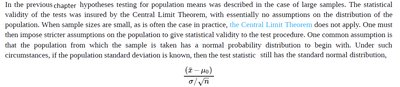
Hypothesis testing is a statistical method used to make inferences about population parameters based on sample data. When the population standard deviation is unknown and the sample size is small (n < 30), the Student's t-distribution is used instead of the normal (z) distribution.
Level of significance (\( \alpha \)): The probability of rejecting the null hypothesis when it is true (Type I error).
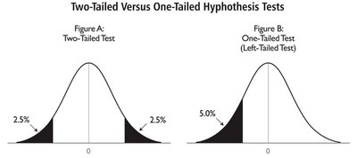
One-tailed vs. Two-tailed tests: Determines the directionality of the test.
Student's t-Distribution
Origin and Purpose
The Student's t-distribution was developed by William S. Gossett, who published under the pseudonym "Student" while working at Guinness Brewery. It is used for hypothesis testing when dealing with small samples and unknown population standard deviation.
Developed for quality control in brewing
Used when sample size is small (n < 30)
Properties of the t-Distribution
The t-distribution is bell-shaped and symmetric about the mean.
It is a family of curves determined by degrees of freedom (df = n - 1).
The mean, median, and mode are all zero.
The total area under the curve is 1 (or 100%).
As degrees of freedom increase, the t-distribution approaches the standard normal (z) distribution.
The t-distribution has thicker tails than the normal distribution, reflecting greater variability in small samples.

Degrees of Freedom
Degrees of freedom (df) refer to the number of independent values that can vary in an analysis without violating any constraints. For a sample of size n, df = n - 1 because one degree is lost in estimating the sample mean.
Example: If you have 7 hats and must wear each once, you have 6 degrees of freedom in choosing the order for the first 6 days; the last day is determined.
t-Test Statistic for Small Samples
When to Use the t-Test
Sample size n < 30
Population standard deviation (\( \sigma \)) is unknown
Population is normally distributed or approximately normal
The t-test statistic is calculated as:
\( \bar{x} \): sample mean
\( \mu \): population mean (under H0)
\( s \): sample standard deviation
\( n \): sample size
Steps in Hypothesis Testing Using the t-Test
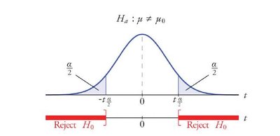
State the hypotheses: Null hypothesis (H0) and alternative hypothesis (Ha).
Specify the significance level (\( \alpha \)).
Calculate degrees of freedom: df = n - 1.
Find the critical value(s): Use the t-table for the given df and \( \alpha \).
Compute the test statistic (t): Use the formula above.
Make a decision: Compare the test statistic to the critical value(s) to decide whether to reject H0.
Interpret the result: State the conclusion in the context of the original claim.
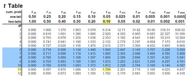
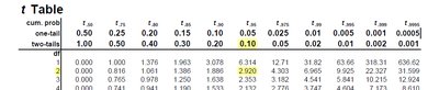
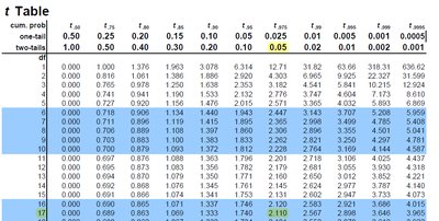
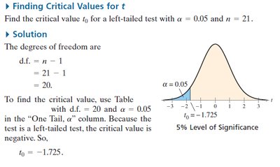
Finding Critical Values in the t-Distribution
Using the t-Table
Identify the significance level (\( \alpha \)) and whether the test is one-tailed or two-tailed.
Find the row for the correct degrees of freedom (df = n - 1).
Read the critical value from the appropriate column (one-tail or two-tail).
Examples of Finding Critical Values
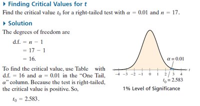
Right-tailed test: \( \alpha = 0.01, n = 17 \), df = 16, t0 = 2.583
Left-tailed test: \( \alpha = 0.05, n = 21 \), df = 20, t0 = -1.725
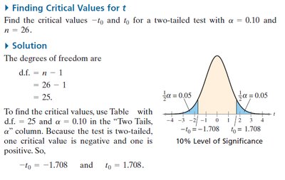
Two-tailed test: \( \alpha = 0.10, n = 26 \), df = 25, t0 = ±1.708
Worked Examples
Example 1: Testing a Mean with a Small Sample
A local telephone company claims the average length of a phone call is 8 minutes. In a random sample of 18 calls, the sample mean is 7.8 minutes, and the standard deviation is 0.5 minutes. Test at \( \alpha = 0.05 \).
H0: \( \mu = 8 \)
Ha: \( \mu \neq 8 \) (two-tailed test)
df = 17, critical values: ±2.110
t = \( \frac{7.8 - 8}{0.5 / \sqrt{18}} \approx -1.70 \)
Decision: -1.70 is within the non-rejection region (between -2.110 and 2.110), so fail to reject H0.
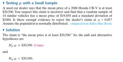
Example 2: Testing a Mean Price (Left-Tailed Test)
A used car dealer claims the mean price of a 2008 Honda CR-V is at least $20,500. A sample of 14 vehicles has a mean of $19,850 and a standard deviation of $1,084. Test at \( \alpha = 0.05 \).
H0: \( \mu \geq 20,500 \)
Ha: \( \mu < 20,500 \) (left-tailed test)
df = 13, critical value: -1.771
t = \( \frac{19,850 - 20,500}{1084 / \sqrt{14}} \approx -2.244 \)
Decision: -2.244 < -1.771, so reject H0.
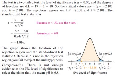
Example 3: Testing a Mean pH Level (Two-Tailed Test)
An industrial company claims the mean pH level of a river is 6.8. A sample of 19 water samples has a mean of 6.7 and a standard deviation of 0.24. Test at \( \alpha = 0.05 \).
H0: \( \mu = 6.8 \)
Ha: \( \mu \neq 6.8 \) (two-tailed test)
df = 18, critical values: ±2.101
t = \( \frac{6.7 - 6.8}{0.24 / \sqrt{19}} \approx -1.816 \)
Decision: -1.816 is within the non-rejection region, so fail to reject H0.
Summary Table: When to Use z-Test vs. t-Test
Condition | Test to Use |
|---|---|
Population standard deviation (\( \sigma \)) known, population normal or n ≥ 30 | z-test |
Population standard deviation (\( \sigma \)) unknown, n ≥ 30 | t-test (approximates z-test) |
Population standard deviation (\( \sigma \)) unknown, n < 30, normal population | t-test |
Population standard deviation (\( \sigma \)) unknown, n < 30, non-normal population | Transform data or use nonparametric test |
Key Formulas
t-test statistic:
Degrees of freedom:
