Hypothesis Testing for Two Means (Dependent Samples) and Two Variances

Two Means from Dependent or Paired Samples

Introduction to Dependent Samples

When comparing two population means, it is common to encounter situations where the samples are dependent. Dependent samples, also known as paired samples, arise when each observation in one sample can be paired with an observation in the other sample based on some relationship (e.g., before/after measurements, matched subjects, or related individuals).

• Key Terms:

  • d: The individual difference between the two values in a matched pair.

  • \( \mu_d \): The population mean of the differences of all matched pairs.

  • \( \overline{d} \): The sample mean of the differences in the sample.

  • \( s_d \): The sample standard deviation of the differences.

  • n: The number of pairs in the sample.

• Example Applications: Measuring honesty in self-reported weights, comparing heights of fathers and sons, before/after treatment effects.

Hypothesis Testing for Dependent Means

To test claims about two population means from dependent samples, we use the following hypothesis test:

• Null Hypothesis (\( H_0 \)): \( \mu_d = 0 \) (no difference in means)

• Alternative Hypothesis (\( H_a \)): \( \mu_d \neq 0 \), \( \mu_d > 0 \), or \( \mu_d < 0 \) (depending on the claim)

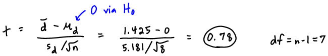
The test statistic is:

$t = \frac{\overline{d} - \mu_d}{s_d / \sqrt{n}}$

This statistic follows a t-distribution with \( df = n - 1 \).

• Requirements:

  • Samples are dependent and randomly selected.

  • Either \( n > 30 \) or the differences are approximately normally distributed.

Confidence Intervals for the Mean Difference

To estimate the mean difference \( \mu_d \) between two dependent samples, construct a confidence interval:

$\overline{d} - E < \mu_d < \overline{d} + E$

where

$E = t_{\alpha/2} \frac{s_d}{\sqrt{n}}$

• If the interval contains 0, there is no significant difference between the means.

• If the interval does not contain 0, the means are likely different.

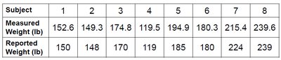
Example: Honesty in Reported Weights

Suppose we want to test if measured weights are higher than reported weights for males. The data below are paired by subject:

• Step (a): The samples are dependent because each measured weight is paired with a reported weight from the same subject.

• Step (b): Hypotheses:

  • \( H_0: \mu_d = 0 \)

  • \( H_a: \mu_d > 0 \) (measured weights are higher)

• Step (c): Calculate \( \overline{d} \), \( s_d \), and \( n \) from the differences.

• Step (d): Compute the test statistic using the formula above.

• Step (e): Use the P-value method to decide whether to reject \( H_0 \).

• Step (f): Use the critical value method for the decision.

• Step (g): Construct the confidence interval for \( \mu_d \).

• Step (h): Write a conclusion in the context of the claim.

Example: Heights of Fathers and Sons

To test if there is a difference in heights between fathers and their first sons, use paired data:

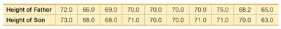
• Follow the same hypothesis testing and confidence interval procedures as above.

The F Distribution and Testing Two Variances

Introduction to the F Distribution

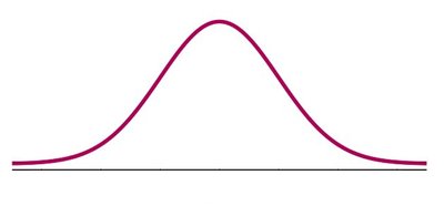
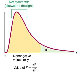
The F distribution is used to compare two population variances or standard deviations. It is a continuous, asymmetric distribution that depends on two degrees of freedom: one for the numerator and one for the denominator.

• Key Properties:

  • Nonnegative values only (variance cannot be negative).

  • Skewed to the right, especially for small sample sizes.

  • As degrees of freedom increase, the F distribution approaches normality.

Hypothesis Testing for Two Variances or Standard Deviations

To test claims about two population variances or standard deviations, use the following hypotheses:

• Null Hypothesis (\( H_0 \)): \( \sigma_1^2 = \sigma_2^2 \) or \( \sigma_1 = \sigma_2 \)

• Test Statistic:

  $F = \frac{s_1^2}{s_2^2}$

  • \( s_1^2 \): Larger sample variance (numerator)

  • \( s_2^2 \): Smaller sample variance (denominator)

  • \( df_1 = n_1 - 1 \), \( df_2 = n_2 - 1 \)

• Requirements:

  • Samples are independent and randomly selected.

  • Both populations are normally distributed.

Interpretation:

• If \( F \approx 1 \), evidence supports equal variances.

• If \( F \gg 1 \), evidence suggests variances are different.

P-values and Critical Values for the F Distribution

• Right-tailed test: Use the right tail of the F distribution.

• Excel functions:

  • P-value (right-tailed): F.DIST.RT(F, df1, df2)

  • P-value (two-tailed): 2*F.DIST.RT(F, df1, df2)

  • Critical value (right-tailed): F.INV.RT(alpha, df1, df2)

  • Critical value (two-tailed): F.INV.RT(alpha/2, df1, df2)

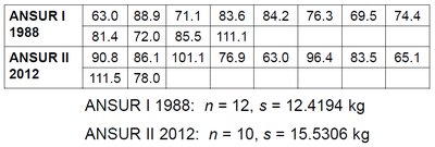
Example: Comparing Variances in Army Personnel Weights

Suppose we want to test if the variation in weights of U.S. Army male personnel changed from 1988 to 2012. The sample statistics are:

• Assign population 1 as the group with the larger sample variance.

• Calculate the F statistic and compare to the critical value or use the P-value method.

• Conclusion: If we fail to reject \( H_0 \), there is not sufficient evidence to claim the variances are different.

Example: Comparing Variances in Penny Weights

To test if the variation in penny weights before 1983 is greater than after 1983, use the following sample statistics:

• Follow the same F-test procedure as above.

Summary Table: Key Differences Between t and F Tests

Test	Purpose	Statistic	Distribution
t-test (paired)	Compare means of dependent samples	$t = \frac{\overline{d} - \mu_d}{s_d / \sqrt{n}}$	t-distribution (df = n-1)
F-test	Compare variances of two independent samples	$F = \frac{s_1^2}{s_2^2}$	F-distribution (df1, df2)

Additional info: The examples and procedures above are foundational for inferential statistics, especially in experimental and observational studies where comparing means and variances is essential for drawing conclusions about populations.