Inference on the Least-Squares Regression Model: Hypothesis Testing, Confidence Intervals, and Model Assumptions

Inference on the Least-Squares Regression Model

Requirements of the Least-Squares Regression Model

The least-squares regression model is a foundational tool in statistics for modeling the linear relationship between an explanatory variable (x) and a response variable (y). For valid inference, several requirements must be met:

• Linearity: For any value of x, the mean of the response variable y depends linearly on x. This is expressed as $\mu_{y|x} = \beta_1 x + \beta_0$.

• Normality and Constant Variance: The response variable y is normally distributed with a constant standard deviation $\sigma$ for each value of x. The mean changes at a constant rate (the slope), while the standard deviation remains constant.

• Independence: The error terms $\varepsilon_i$ are independent and have mean zero and constant variance $\sigma^2$.

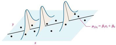
Interpretation: A large value of $\sigma$ indicates data are widely dispersed about the regression line, while a small $\sigma$ means data are close to the line.

The Least-Squares Regression Model Equation

• The model is given by $y_i = \beta_1 x_i + \beta_0 + \varepsilon_i$, where $\varepsilon_i$ is a random error term with mean 0 and variance $\sigma^2$.

• Parameters $\beta_0$ (intercept) and $\beta_1$ (slope) are estimated from sample data.

Standard Error of the Estimate

The standard error of the estimate ($s_e$) measures the typical distance that the observed values fall from the regression line. It is calculated as:

• $s_e = \sqrt{\dfrac{\sum (y_i - \hat{y}_i)^2}{n-2}}$

• Where $y_i$ is the observed value, $\hat{y}_i$ is the predicted value, and $n$ is the sample size.

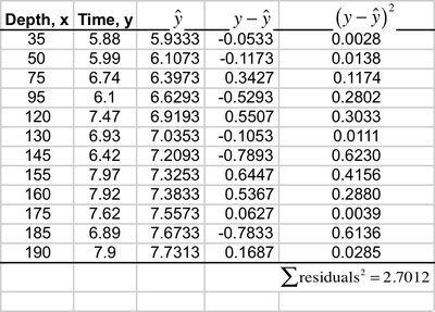
Example: For the drilling data, $\sum (y_i - \hat{y}_i)^2 = 2.7012$ and $n = 12$, so $s_e = \sqrt{2.7012/10} = 0.5197$.

Note: Always divide by $n-2$ when computing $s_e$ for regression.

Verifying Normality of Residuals

To ensure valid inference, the residuals (differences between observed and predicted values) should be approximately normally distributed. This can be checked using a normal probability plot.

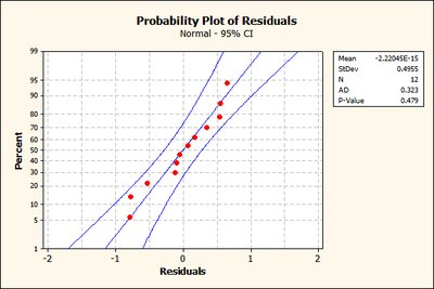
Interpretation: If the residuals fall approximately along a straight line in the probability plot, the normality assumption is reasonable.

Hypothesis Testing for the Slope

To determine if there is a significant linear relationship between x and y, we test hypotheses about the slope $\beta_1$:

• Null hypothesis ($H_0$): $\beta_1 = 0$ (no linear relationship)

• Alternative hypothesis ($H_1$): $\beta_1 \neq 0$, $\beta_1 < 0$, or $\beta_1 > 0$ (depending on the research question)

The test statistic is:

• $t_0 = \dfrac{b_1 - \beta_1}{s_{b_1}} = \dfrac{b_1}{s_{b_1}}$ (since $\beta_1 = 0$ under $H_0$)

• $s_{b_1} = \dfrac{s_e}{\sqrt{\sum (x_i - \bar{x})^2}}$

This statistic follows a Student's t-distribution with $n-2$ degrees of freedom.

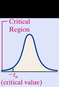
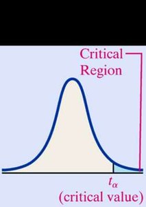
Critical Value Approach

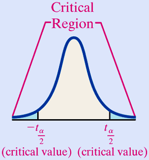
Compare the calculated $t_0$ to the critical value(s) from the t-distribution:

Test Type	Decision Rule
Two-Tailed	If $t_0 < -t_{\alpha/2}$ or $t_0 > t_{\alpha/2}$, reject $H_0$.
Left-Tailed	If $t_0 < -t_{\alpha}$, reject $H_0$.
Right-Tailed	If $t_0 > t_{\alpha}$, reject $H_0$.

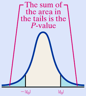
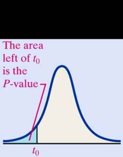
P-Value Approach

The P-value is the probability, under $H_0$, of observing a test statistic as extreme as, or more extreme than, the value computed from the sample.

• For a two-tailed test, the P-value is the sum of the areas in both tails beyond $|t_0|$.

• For a left-tailed test, it is the area to the left of $t_0$.

• For a right-tailed test, it is the area to the right of $t_0$.

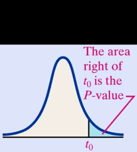
Decision Rule: If the P-value < $\alpha$, reject $H_0$.

Checking Model Assumptions with Residual Plots

Before conducting inference, check that the residuals show no pattern when plotted against the explanatory variable. This supports the assumption of constant variance (homoscedasticity).

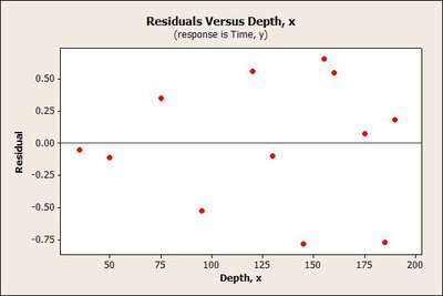
Interpretation: No discernable pattern indicates the model assumptions are reasonable.

Calculating the Standard Error of the Slope

The standard error of the slope estimate $s_{b_1}$ is calculated as:

• $s_{b_1} = \dfrac{s_e}{\sqrt{\sum (x_i - \bar{x})^2}}$

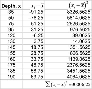
Example: For the drilling data, $s_e = 0.5197$ and $\sum (x_i - \bar{x})^2 = 30006.25$, so $s_{b_1} = 0.0030$.

Constructing a Confidence Interval for the Slope

A $(1-\alpha)\times 100\%$ confidence interval for the true slope $\beta_1$ is:

• Lower bound: $b_1 - t_{\alpha/2} \cdot s_{b_1}$

• Upper bound: $b_1 + t_{\alpha/2} \cdot s_{b_1}$

Example: For $b_1 = 0.0116$, $s_{b_1} = 0.0030$, $t_{0.025} = 2.228$ (10 df):

• Lower bound: $0.0116 - 2.228 \times 0.003 = 0.0049$

• Upper bound: $0.0116 + 2.228 \times 0.003 = 0.0183$

We are 95% confident that the true mean increase in time to drill 5 feet for each additional foot of depth is between 0.005 and 0.018 minutes.

Confidence and Prediction Intervals for the Regression Model

These intervals provide measures of accuracy for predictions made using the regression model:

• Confidence Interval for Mean Response: Estimates the mean value of y for all individuals at a specific x.

• Prediction Interval for Individual Response: Estimates the value of y for a single individual at a specific x.

Formulas:

• Confidence interval for mean response at $x^*$: Lower: $\hat{y} - t_{\alpha/2} \cdot s_e \sqrt{\dfrac{1}{n} + \dfrac{(x^* - \bar{x})^2}{\sum (x_i - \bar{x})^2}}$ Upper: $\hat{y} + t_{\alpha/2} \cdot s_e \sqrt{\dfrac{1}{n} + \dfrac{(x^* - \bar{x})^2}{\sum (x_i - \bar{x})^2}}$

• Prediction interval for individual response at $x^*$: Lower: $\hat{y} - t_{\alpha/2} \cdot s_e \sqrt{1 + \dfrac{1}{n} + \dfrac{(x^* - \bar{x})^2}{\sum (x_i - \bar{x})^2}}$ Upper: $\hat{y} + t_{\alpha/2} \cdot s_e \sqrt{1 + \dfrac{1}{n} + \dfrac{(x^* - \bar{x})^2}{\sum (x_i - \bar{x})^2}}$

Example: For $x^* = 110$, $\hat{y} = 6.8033$, $s_e = 0.5197$, $n = 12$, $\bar{x} = 126.25$, $\sum (x_i - \bar{x})^2 = 30006.25$, $t_{0.025} = 2.228$:

• Confidence interval for mean response: (6.45, 7.15)

• Prediction interval for individual response: (5.59, 8.01)

We are 95% confident that the mean time to drill 5 feet at 110 feet depth is between 6.45 and 7.15 minutes, and for a single drilling, the time is between 5.59 and 8.01 minutes.