Inference on the Least-Squares Regression Model and Multiple Regression

Chapter 14: Inference on the Least-Squares Regression Model and Multiple Regression

Section 14.1: Testing the Significance of the Least-Squares Regression Model

This section introduces the process of making statistical inferences about the least-squares regression model, focusing on the requirements, computation, and hypothesis testing for the slope coefficient.

Learning Objectives

• State the requirements of the least-squares regression model.

• Compute the standard error of the estimate.

• Verify that the residuals are normally distributed.

• Conduct inference on the slope of the least-squares regression model.

• Construct a confidence interval about the slope of the least-squares regression model.

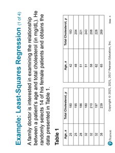
Example: Least-Squares Regression

This example examines the relationship between age and total cholesterol in female patients. The data are presented in a table and analyzed using least-squares regression techniques.

Age, x	Total Cholesterol, y
25	180
28	186
31	195
35	200
38	210
42	220
45	225
48	230
51	235
55	239
58	250
61	260
65	270
68	280

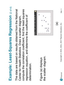
The scatter diagram and regression output are used to find the least-squares regression equation and the coefficient of determination.

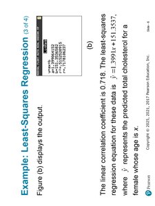
• Regression Equation: $\hat{y} = 1.399x + 151.357$

• Correlation Coefficient: $r = 0.718$

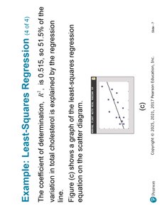
• Coefficient of Determination: $R^2 = 0.515$ (51.5% of the variation in cholesterol is explained by age)

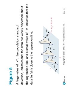
Requirements for Inference on the Least-Squares Regression Model

• Linearity: For any value of the explanatory variable $x$, the mean response $\mu_y$ is a linear function of $x$: \mu_y = \beta_1 x + \beta_0 $ $ where $\beta_1$ and $\beta_0$ are population parameters.

• Normality: The response variable is normally distributed with mean $\mu_y = \beta_1 x + \beta_0$ and standard deviation $\sigma$.

Interpretation: The mean response changes linearly with $x$, while the standard deviation remains constant. A large $\sigma$ indicates data are widely dispersed about the regression line; a small $\sigma$ means data are close to the line.

Definitions

• Least-Squares Regression Model: y_i = \beta_1 x_i + \beta_0 + \varepsilon_i $ $ where $y_i$ is the response, $x_i$ is the explanatory variable, $\beta_1$ and $\beta_0$ are parameters, and $\varepsilon_i$ is the random error.

• Standard Error of the Estimate ($s_e$): s_e = \sqrt{\frac{\sum (y_i - \hat{y}_i)^2}{n-2}} $ $ where $\hat{y}_i$ are the predicted values and $n$ is the sample size.

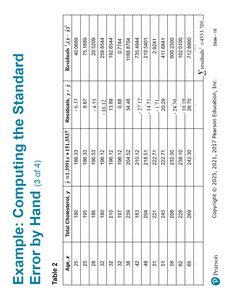
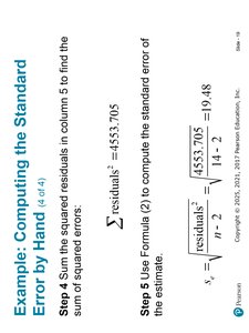
Example: Computing the Standard Error by Hand

To compute the standard error, use the observed and predicted values to find the residuals, square them, sum them, and apply the formula above.

Example: Obtaining the Standard Error Using Technology

Statistical software can be used to compute the standard error, which should match the hand calculation.

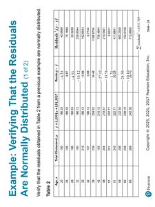
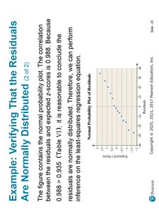
Verifying That the Residuals Are Normally Distributed

To perform inference, residuals must be approximately normally distributed. This can be checked using a normal probability plot and by comparing the correlation between residuals and expected z-scores to a critical value.

Conducting Inference on the Slope of the Least-Squares Regression Model

Hypothesis tests are used to determine if there is a significant linear relationship between two quantitative variables.

• Null Hypothesis ($H_0$): $\beta_1 = 0$ (no linear relationship)

• Alternative Hypothesis ($H_1$): $\beta_1 \neq 0$, $\beta_1 > 0$, or $\beta_1 < 0$ (depending on the test)

Test Type	Null Hypothesis	Alternative Hypothesis
Two-tailed	$\beta_1 = 0$	$\beta_1 \neq 0$
Right-tailed	$\beta_1 = 0$	$\beta_1 > 0$
Left-tailed	$\beta_1 = 0$	$\beta_1 < 0$

Test Statistic: t = \frac{b_1}{s_{b_1}} $ $ where $b_1$ is the sample slope and $s_{b_1}$ is its standard error. The test statistic follows a t-distribution with $n-2$ degrees of freedom.

Classical Approach

1. Compute the test statistic.

2. Determine the critical value from the t-distribution.

3. Compare the test statistic to the critical value and state the conclusion.

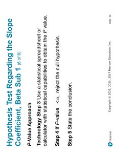
P-Value Approach

1. Compute the test statistic.

2. Use statistical software or tables to find the p-value.

3. If p-value < $\alpha$, reject the null hypothesis.

4. State the conclusion.

Caution

Before testing $H_0: \beta_1 = 0$, always draw a residual plot to verify that a linear model is appropriate.

Example: Testing for a Linear Relation

To test for a linear relationship between age and cholesterol at $\alpha = 0.05$, follow these steps:

1. State hypotheses: $H_0: \beta_1 = 0$ vs. $H_1: \beta_1 \neq 0$

2. Set significance level: $\alpha = 0.05$

3. Compute the test statistic using the sample data and standard error.

4. Compare to the critical value or use the p-value approach.

5. Draw a conclusion about the existence of a linear relationship.

Summary: This section provides a comprehensive approach to testing the significance of the least-squares regression model, including requirements, computation of standard error, verification of normality, and hypothesis testing for the slope coefficient.