Introduction to Data and Visualizing Data in Statistics

Study Guide - Smart Notes

Tailored notes based on your materials, expanded with key definitions, examples, and context.

Introduction to Statistics and Data

What is Statistics?

Statistics is the science of collecting, organizing, summarizing, and analyzing data to answer questions and draw conclusions. It is widely used in various fields such as biology, exercise science, social sciences, and business.

Data: Observations gathered to draw conclusions. Examples include the weight of children in kilograms or the percentage of honey bee wintering losses in a province.
Variation: Differences or changes in an item or variable. Variation is a fundamental concept in statistics, as it helps us understand the diversity and patterns within data.

Variables

A variable is a characteristic of people or things that can take on different values from individual to individual.

Examples: Weight of a newborn baby, price of a litre of gas, ground-level ozone concentration in the air.
The value of a variable can change from one individual to another.

Population vs. Sample

Understanding the difference between a population and a sample is crucial in statistics.

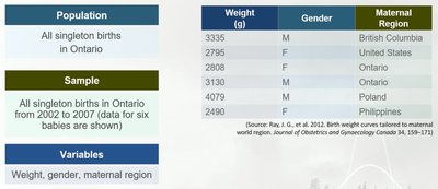
Population: The collection of all possible data values for the variable of interest. Gathering data from the entire population is often difficult, time-consuming, and costly.
Sample: A subset of the population. Information is easier and less costly to collect from a sample. Inferential statistics allow us to learn about the population by studying the sample.

Population, Sample, and Variables table with birth weights example

Data Collection Context

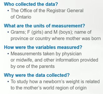
Who collected the data? The Office of the Registrar General of Ontario.
Units of measurement: Grams (weight), F (girls) and M (boys) for gender, and the name of the province or country for maternal region.
How were variables measured? Measurements taken by physician or midwife; other information provided by a parent.
Purpose: To study how a newborn’s weight is related to the mother’s world region of origin.

Data collection context: who, what, how, and why

Classifying Variables and Data

Types of Variables

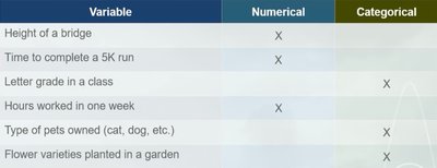
Numerical Variables: Describe a quantity or measurement. Values are numbers (e.g., temperature, salary, number of kittens in a litter).
Categorical Variables: Describe qualities or categories (e.g., eye color, diabetes status, level of agreement with a statement). Values are categories, such as Yes or No.

Table classifying variables as numerical or categorical

Coding Categorical Data

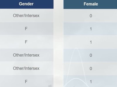
Categorical data can be coded using numbers to make data storage and analysis easier. For example, gender may be coded as 1 for female and 0 for not female. These numbers do not represent quantities.

Coding categorical data example: Gender and Female columns

Stacked vs. Unstacked Data

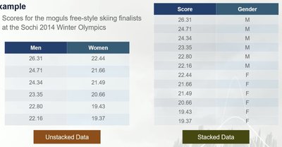
Stacked Data: Data values are stored in a spreadsheet format where each row contains data for a single individual and can store many variables.
Unstacked Data: Data values are stored in two or more columns, each representing a variable from a group. Can only store data for two variables.

Stacked and unstacked data example with Olympic scores

Organizing and Displaying Data

Why Organize Data?

Organizing data helps us see patterns and make sense of the information. Displaying data visually is not always straightforward but is essential for analysis.

Two-Way Tables

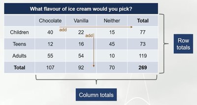
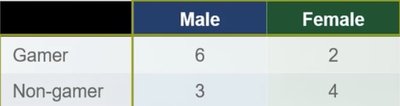
Two-way tables are a common way to organize categorical data, displaying results from two potentially related categorical variables and showing the frequency of each combination.

Two-way table: ice cream flavor preference by age group Two-way table: gamer status by gender

Comparing Data: Counts vs. Percentages

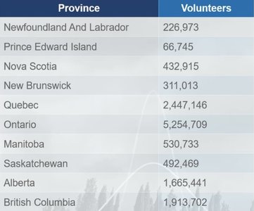
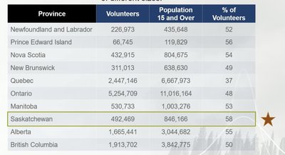
Percentages or rates are better than counts for making comparisons between groups of different sizes. For example, to compare volunteer rates across provinces, it is important to consider the population size.

Table of volunteers by province (counts only)

Studying Causality and Experimental Design

Treatment and Outcome Variables

Treatment Variable: Whether or not a specific treatment is used.
Outcome Variable: The response to changes in the treatment.
Goal: To determine whether changes in the treatment variable cause changes in the outcome variable.

Methods for Collecting Data

Anecdotal Evidence: Based on personal stories or experiences; not reliable for drawing scientific conclusions.
Observational Study: Subjects are placed in groups by choice or circumstances not controlled by the researcher. Can establish relationships but not causality.
Controlled Experiment: Researchers assign subjects to treatment and control groups, allowing for causal inference if well-designed.

Correlation vs. Causation

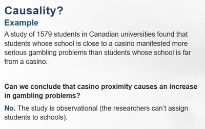
Only well-designed controlled experiments can establish causality. Observational studies can only show associations, not cause-and-effect relationships.

Causality example: casino proximity and gambling problems

Confounding Variables

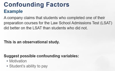
A confounding variable is an alternative explanation for observed differences between groups. It cannot be ruled out in observational studies.

Confounding factors example: LSAT preparation

Gold Standard for Experiments

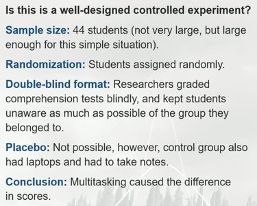
Large sample size to account for variability
Random assignment to treatment or control group to minimize bias
Use of placebo if appropriate
Double-blind study design to avoid bias

Case Study: Multitasking in the Classroom

An experiment with 44 university students showed that multitasking students scored 11% lower on comprehension tests than the control group. The study used randomization and blind grading, supporting a causal conclusion.

Experiment: multitasking in the classroom Controlled experiment design: sample size, randomization, double-blind, placebo, conclusion

Describing Data with Tables and Graphs

What is a Distribution?

A distribution records all observed values (numbers or categories) and their frequencies. Graphs help visualize patterns in the data.

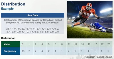
Distribution example: CFL touchdown passes raw data and frequency table

Dotplots

Each observation is represented by a dot on a number line. Dotplots are most useful for small data sets.

Dotplot example

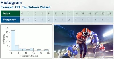
Histograms

Observations are grouped into intervals (bins), and each bin is represented by a vertical bar. The height of the bar is proportional to the frequency of observations in that bin.

Changing the bin width changes the appearance of the histogram. Thinner bins give more detail; wider bins give less.
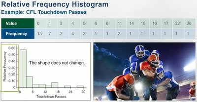
Relative frequency histograms show the proportion of observations in each bin. The shape does not change compared to the frequency histogram.

Histogram example: CFL touchdown passes Relative frequency histogram example: CFL touchdown passes

Stemplots

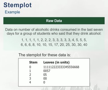
Stemplots (or stem-and-leaf plots) show all individual data values in a compact form. The last digit is the leaf, and all preceding digits make the stem. Useful for small data sets or when technology is not available.

Stemplot example: number of alcoholic drinks

Describing Numerical Distributions

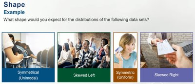
Shape

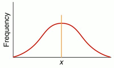
Symmetric: Left and right sides of the graph are roughly the same.
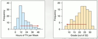
Skewed: Most data is on one side with a long tail on the other.
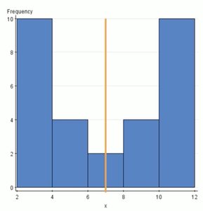
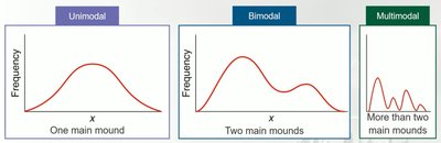
Mounds: The number of peaks or mounds in the distribution (unimodal, bimodal, multimodal).
Outliers: Extremely large or small values that do not fit the pattern of the rest of the data. Outliers should be reported and investigated further.

Symmetric distribution example Uniform distribution example Skewed distributions example Unimodal, bimodal, and multimodal distributions Shape examples: symmetrical, skewed left, symmetric uniform, skewed right

Center

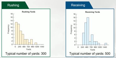
The center of a distribution is the typical data value. For example, histograms of total rushing and receiving yards for football players show different typical values.

Histograms of rushing and receiving yards

Variability (Spread)

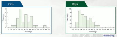
Variability refers to the horizontal spread of the data. Wide graphs indicate high variability; narrow graphs indicate low variability.

Histograms showing variability in vegetable consumption for girls and boys

Describing Categorical Distributions

Bar Charts

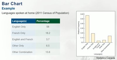
Bar charts display data categories on the horizontal axis, with bars representing the frequency or relative frequency of each category. Categories can be ordered in various ways.

Bar chart example: languages spoken at home

Pie Charts

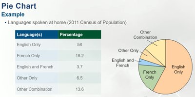
Pie charts show the proportion of observations in each category as wedges of a circle. Although common, pie charts are generally not recommended by statisticians due to difficulty in comparing areas accurately.

Pie chart example: languages spoken at home

Bar Chart vs. Histogram

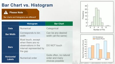
	Histogram	Bar Chart
Data	Numerical	Categorical
Bar Width	Corresponds to bin width	Any desired width (all the same)
Bars	Must touch, except when there are no observations in the interval	Do NOT touch
Horizontal Labels	Numerical order	No natural order; many choices possible

Bar chart vs. histogram comparison

Mode and Variability in Categorical Data

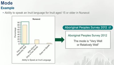
Mode: The category that occurs most often. For categorical data, modes must be roughly the same height.
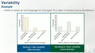
Variability: Diversity in the data values. High variability means many observations in many categories; low variability means many observations in only a few categories.

Mode example: ability to speak an Inuit language Variability example: ability to speak an Inuit language in two regions

Misleading Graphs

Common Errors in Graphs

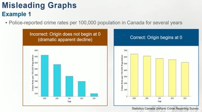
Frequency scale not beginning at zero, creating the illusion of greater differences
Shading or 3D effects that convey no information
Use of drawings instead of bars, which can hide or accentuate real differences
Axes with non-constant scale

Misleading graphs: origin not at zero vs. correct origin

Note: Raw data are ineffective for making comparisons; visual summaries are essential for clear communication.