Introduction to Probability Theory: Experiments, Counting, and Probability Laws

Introduction to Probability Theory

Probability theory provides a mathematical framework for quantifying uncertainty and making informed decisions in the presence of randomness. It is widely used in science, business, and everyday life to assess the likelihood of various outcomes.

Experiments, Counting Rules, and Assigning Probabilities

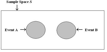
Experiments and Sample Spaces

An experiment is a process that produces well-defined outcomes. The sample space (denoted as S) is the set of all possible outcomes of an experiment. Each outcome is called a sample point.

• Example: Rolling a die: S = {1, 2, 3, 4, 5, 6}

• Example: Tossing a coin: S = {Head, Tail}

• Example: Selecting a part: S = {Defective, Non-defective}

Counting Rules, Combinations, and Permutations

Counting the number of possible outcomes is essential for assigning probabilities. Several rules are used:

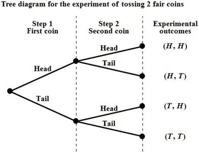
• Multiple-Step Experiments: If an experiment consists of k steps with n1, n2, ..., nk possible outcomes at each step, the total number of outcomes is n1 × n2 × ... × nk.

Example: Tossing two coins (each with 2 outcomes): 2 × 2 = 4 outcomes.

• Factorials (!): The product of all positive integers up to n. Used for arrangements where order matters and no repetitions are allowed. $n! = n \times (n-1) \times (n-2) \times \ldots \times 1$

• Combinations: The number of ways to choose n objects from N without regard to order: $C_N^n = \frac{N!}{n!(N-n)!}$ Order does not matter.

• Permutations: The number of ways to arrange n objects from N where order matters: $P_N^n = \frac{N!}{(N-n)!}$ Order matters.

Assigning Probabilities

Probabilities can be assigned using three main approaches:

1. Classical Method: Used when all outcomes are equally likely. Each outcome has probability $\frac{1}{n}$.

2. Relative Frequency Method: Based on observed data; probability is estimated as the proportion of times an outcome occurs in repeated trials.

3. Subjective Method: Based on personal judgment or experience when data is insufficient or outcomes are not equally likely.

Requirements for Probabilities:

• All probabilities must be between 0 and 1: $0 \leq P(E_i) \leq 1$

• The sum of probabilities for all outcomes must equal 1: $P(E_1) + P(E_2) + \ldots + P(E_n) = 1$

Basic Relationships of Probability

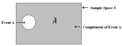
Complement of an Event

The complement of event A (denoted Ac or \( \overline{A} \)) consists of all outcomes not in A. The probability of the complement is:

• $P(A^c) = 1 - P(A)$

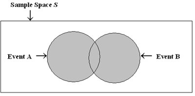
Union of Two Events

The union of events A and B (A ∪ B) is the event that either A or B or both occur.

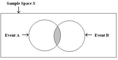
Intersection of Two Events

The intersection of events A and B (A ∩ B) is the event that both A and B occur.

Addition Law

The addition law calculates the probability that at least one of two events occurs:

• $P(A \cup B) = P(A) + P(B) - P(A \cap B)$

This formula corrects for double-counting the intersection of A and B.

Mutually Exclusive Events

Events are mutually exclusive if they cannot occur together (i.e., $P(A \cap B) = 0$). For such events:

• $P(A \cup B) = P(A) + P(B)$

Other Probability Laws

• Commutative Laws: $A \cup B = B \cup A$, $A \cap B = B \cap A$

• Associative Laws: $(A \cup B) \cup C = A \cup (B \cup C)$, $(A \cap B) \cap C = A \cap (B \cap C)$

• DeMorgan’s Laws: $(A \cap B)^c = A^c \cup B^c$, $(A \cup B)^c = A^c \cap B^c$

Conditional Probability

The conditional probability of event A given event B has occurred is:

• $P(A|B) = \frac{P(A \cap B)}{P(B)}$

This measures the probability of A under the condition that B is known to have occurred.

Example: Employee Promotion Table

Gender	Promoted (Yes)	Promoted (No)	Total
Male	288	672	960
Female	36	204	240
Total	324	876	1200

Probabilities can be calculated as follows:

• Marginal probability (e.g., probability of being promoted): $P(A) = \frac{324}{1200} = 0.27$

• Joint probability (e.g., probability of being male and promoted): $P(M \cap A) = \frac{288}{1200} = 0.24$

• Conditional probability (e.g., probability of being promoted given male): $P(A|M) = \frac{288/1200}{960/1200} = \frac{288}{960} = 0.3$

Independence of Events

Events A and B are independent if the occurrence of one does not affect the probability of the other:

• $P(A|B) = P(A)$ or $P(B|A) = P(B)$

• Alternatively, $P(A \cap B) = P(A)P(B)$

If these equalities do not hold, the events are dependent.

Multiplication Law

The multiplication law is used to find the probability of the intersection of two events:

• $P(A \cap B) = P(B)P(A|B)$ or $P(A \cap B) = P(A)P(B|A)$

• If A and B are independent: $P(A \cap B) = P(A)P(B)$

Summary Table: Joint and Marginal Probabilities

Gender	Promoted (Yes)	Promoted (No)	Total
Male	0.24	0.56	0.8
Female	0.03	0.17	0.2
Total	0.27	0.73	1

Example: If $P(L) = 0.3$ and $P(C) = 0.08$ are independent, then $P(L \cup C) = P(L) + P(C) - P(L)P(C) = 0.356$.

Additional info: These foundational probability concepts are essential for further study in statistics, including probability distributions, inferential statistics, and regression analysis.