Introduction to Statistics: Data, Variables, and the Five W’s

Study Guide - Smart Notes

Tailored notes based on your materials, expanded with key definitions, examples, and context.

Section 1.2: Data and the Five W’s and H

Understanding Data Collection

To analyze any data set, it is crucial to identify the context in which the data were collected. This is summarized by the Five W’s and one H:

Who: The subjects or cases being studied.
What: The variables measured or recorded.
When: The time period during which the data were collected.
Where: The location or setting of the study.
Why: The purpose or motivation for collecting the data.
How: The method or process used to collect the data.

Who, What, When, Where, Why, How sticky notes

Example: In a study on muscle hypertrophy, researchers collected data on young men performing resistance training to determine the effects of lifting lighter versus heavier weights.

Journal article on resistance training NY Times headline on lifting weights

Components of a Data Set

A data set consists of cases (rows) and variables (columns). Each case provides a set of measurements or responses for the variables of interest.

Cases: The individual units or subjects from which data are collected.
Variables: The characteristics or attributes measured for each case.

Section 1.3: Variables and Their Types

Identifying Variables

Variables are characteristics or attributes that can take on different values among cases in a data set. Understanding the type of variable is essential for choosing appropriate statistical methods.

Variability: The degree to which data values differ among cases.
Examples of Variables: Size, fur color, weight, eye color, height, breed, collar presence, age, tongue position, ear length, paw size, fur length, name, fastest speed, number of unique fur colors.

Dogs of various breeds and sizes

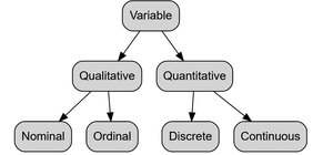
Types of Variables

Categorical Variables (Qualitative): Place cases into groups or categories. Responses are words or labels. Can be nominal (no order) or ordinal (ordered categories).
Quantitative Variables (Numerical): Measured or recorded as numbers. Calculations with these numbers make sense. Can be discrete (countable) or continuous (measurable).

Variable classification diagram

Examples:

Categorical: Size (Small, Medium, Large), Fur Color, Eye Color, Breed, Collar (yes/no), Name, Tongue (out/not), Inversion (yes/no).
Quantitative: Weight (pounds), Height (inches), Age (years), Ear Length (inches), Fur Length (inches), Fastest Speed (miles per hour), Number of unique colors.

Practice: Identifying Variable Types in a Data Set

Given a roller coaster data set with variables such as Name, Park, Type, Duration, Speed, Height, Drop, Length, Inversion, and Number of Inversions, students are asked to classify variables as categorical or quantitative.

Example Answer: 3 categorical variables (Name, Park, Type), 7 quantitative variables (Duration, Speed, Height, Drop, Length, Inversion, Number of Inversions).

Visualizing Data: Graphs and Tables

Different types of graphs are used to display categorical and quantitative data:

Bar Charts: Used for categorical variables to show counts or frequencies.
Scatterplots: Used for quantitative variables to show relationships between two numerical variables.
Boxplots: Used to display the distribution of a quantitative variable for different groups.

Bar chart of place of death Bar chart of roller coaster type Scatterplot of duration vs length

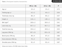
Tables: Describing and Summarizing Data

Tables are used to summarize and compare data across groups or categories. For example, a table of baseline characteristics can show the effectiveness of random assignment in an experiment.

Variable	HR (n = 24)	LR (n = 25)	P
Age, yr	23 ± 2	23 ± 2	0.73
Training age, yr	4.2 ± 2.0	4.6 ± 1.8	0.54
Total body mass, kg	88 ± 4	88 ± 4	0.81
Height, m	1.80 ± 0.1	1.80 ± 0.1	0.81
BMI, kg/m2	26.8 ± 2.1	26.8 ± 2.1	0.99
Lean mass, kg	67.6 ± 7.2	67.9 ± 7.1	0.99
Total fat mass, kg	14.9 ± 2.4	14.8 ± 2.4	0.97
Leg press 1RM, kg	357 ± 25	351 ± 23	0.87
Bench press 1RM, kg	96 ± 13	92 ± 14	0.41
Shoulder press 1RM, kg	91 ± 5	92 ± 4	0.87

Table of baseline characteristics

Special Cases: Recoding Variables

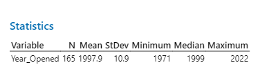
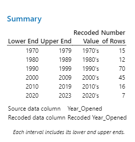
Sometimes, quantitative variables are recoded into categorical variables for analysis. For example, the year a roller coaster opened can be grouped into decades.

Lower End	Upper End	Recoded Value	Number of Rows
1970	1979	1970's	15
1980	1989	1980's	12
1990	1999	1990's	70
2000	2009	2000's	45
2010	2019	2010's	16
2020	2023	2020's	7

Summary table of recoded year opened Chart of recoded year opened

Special Variable Types: Ordinal and Identifier Variables

Ordinal Variables: Categorical variables with a meaningful order (e.g., Likert scale ratings).
Identifier Variables: Unique labels for cases (e.g., ZIP codes), which are categorical but do not have a meaningful order or quantitative interpretation.

Example: ZIP codes are categorical variables used as identifiers, not as ordinal or quantitative variables.

Summary

Statistics is the science of learning from data and making decisions under uncertainty.
Understanding the context of data collection (the Five W’s and H) is essential for proper analysis.
Variables can be categorical or quantitative, and their correct identification is crucial for analysis.
Tables and graphs are fundamental tools for summarizing and visualizing data.
Special variable types include ordinal and identifier variables, which require careful interpretation.