Introductory Statistics: Chapter 4 - Probability Study Notes

Probability

Introduction to Probability

Probability is a fundamental concept in statistics that quantifies how likely an event is to occur. It provides a mathematical framework for making predictions and decisions based on data.

• Probability: How often something occurs or is expected to occur.

• Probability gives us information about data in a widely accessible format.

• Probability theory can be used to make decisions about populations, such as using the Rare Event Rule.

Rare Event Rule for Inferential Statistics

The Rare Event Rule is used in inferential statistics to determine whether an observed event is statistically significant. If the probability of an event is extremely small under a given assumption, the assumption is likely incorrect.

• If, under a given assumption, the probability of an observed event is extremely small, then the assumption is probably not correct.

• Such an event is called statistically significant because it is too unlikely to occur by chance.

• This rule is foundational for hypothesis testing and will be revisited later in the course.

Basic Probability Terms

Key Definitions

Understanding basic probability terms is essential for analyzing and solving probability problems.

• Event: An outcome of a procedure.

• Simple event: An event that cannot be broken down into simpler components.

• Outcome: The result of a single trial in a procedure.

• Sample Space: The set of all possible outcomes of a procedure.

Sample Space and Tree Diagrams

Tree Diagrams

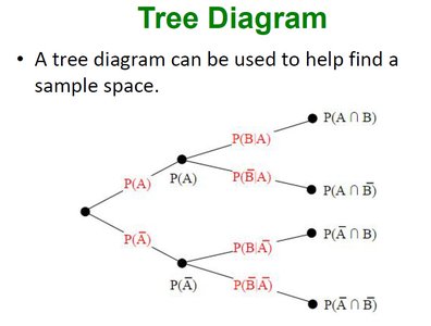
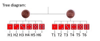
Tree diagrams are visual tools used to systematically list all possible outcomes (sample space) of a probability experiment. They are especially useful for multi-step experiments.

• Each branch represents a possible outcome at each stage.

• Tree diagrams help in finding probabilities of combined events.

Examples of Sample Spaces

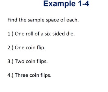
Sample spaces can be constructed for simple experiments such as rolling dice or flipping coins.

• One roll of a six-sided die: {1, 2, 3, 4, 5, 6}

• One coin flip: {Heads, Tails}

• Two coin flips: {HH, HT, TH, TT}

• Three coin flips: {HHH, HHT, HTH, HTT, THH, THT, TTH, TTT}

Complex Sample Spaces

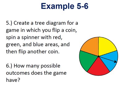
Tree diagrams can be used for more complex experiments, such as games involving coins, spinners, and additional coin flips.

• For a game with a coin flip, a spinner (red, green, blue), and another coin flip, the sample space is constructed by multiplying the outcomes at each stage.

• Number of possible outcomes = 2 (coin) × 3 (spinner) × 2 (coin) = 12

Fundamental Counting Principle

Definition and Application

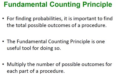
The Fundamental Counting Principle is a method for determining the total number of possible outcomes in a multi-step experiment.

• Multiply the number of possible outcomes for each part of a procedure.

• Useful for calculating probabilities in complex scenarios.

Example: Car Selection

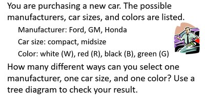
Suppose you are purchasing a new car. The possible manufacturers, car sizes, and colors are listed. The total number of ways to select one manufacturer, one car size, and one color is found by multiplying the number of choices for each category.

• Manufacturers: Ford, GM, Honda (3 choices)

• Car size: compact, midsize (2 choices)

• Color: white, red, black, green (4 choices)

• Total ways = 3 × 2 × 4 = 24

Additional Counting Examples

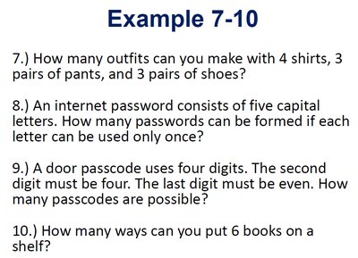
Counting principles can be applied to various scenarios, such as outfits, passwords, passcodes, and arranging books.

• Outfits: 4 shirts × 3 pants × 3 shoes = 36 possible outfits

• Passwords: If each letter is unique, use permutations

• Passcodes: Apply restrictions for digits

• Arranging books: Use factorials

Factorial

Definition and Calculation

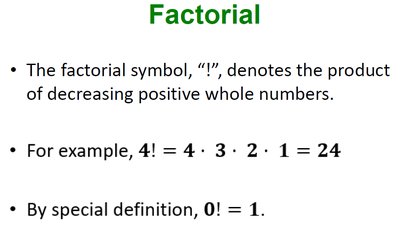
The factorial symbol "!" denotes the product of decreasing positive whole numbers. Factorials are used in counting and probability calculations, especially for permutations.

• For example, $4! = 4 \cdot 3 \cdot 2 \cdot 1 = 24$

• By definition, $0! = 1$

Factorial Examples

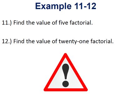
• Find the value of five factorial: $5! = 5 \cdot 4 \cdot 3 \cdot 2 \cdot 1 = 120$

• Find the value of twenty-one factorial: $21!$ (a very large number)

Probability Rules

Basic Rules

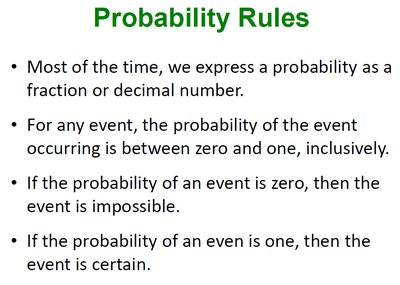
Probabilities are usually expressed as fractions or decimals and must satisfy certain rules.

• For any event, the probability is between 0 and 1, inclusive.

• If the probability is 0, the event is impossible.

• If the probability is 1, the event is certain.

Example: Valid Probabilities

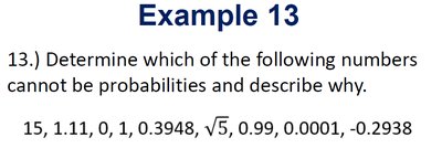
Determine which numbers cannot be probabilities and explain why.

• Valid probabilities: 0, 1, 0.3948, 0.99, 0.0001

• Invalid probabilities: 15, 1.11, $\sqrt{5}$, -0.2938 (because they are not between 0 and 1)

Classical vs. Relative Frequency Probability

Definitions and Comparison

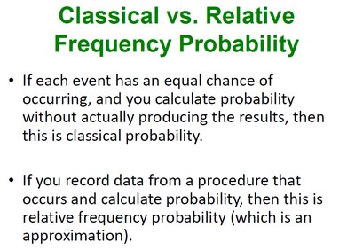
There are two main approaches to calculating probability: classical and relative frequency.

• Classical Probability: Used when each event has an equal chance of occurring and is calculated without actually performing the experiment.

• Relative Frequency Probability: Calculated by recording data from actual experiments; it is an approximation.

Calculating Probability

Probability Formula

The probability of an event A is calculated as the ratio of the number of occurrences of A to the total number of possible outcomes.

• Formula: $P(A) = \frac{\text{number of occurrences of A}}{\text{total number of outcomes}}$

• This formula is fundamental for both classical and empirical probability calculations.

Summary Table: Probability Concepts

Concept	Definition	Example
Event	Outcome of a procedure	Rolling a 4 on a die
Sample Space	All possible outcomes	{1,2,3,4,5,6} for a die
Classical Probability	Equal chance, theoretical	Probability of heads on a coin: 0.5
Relative Frequency	Based on experiment	Observed heads in 100 flips
Factorial	Product of decreasing numbers	4! = 24