Introductory Statistics: Core Concepts and Methods

Introduction to Statistics

What is Statistics?

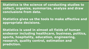
Statistics is the science of conducting studies to collect, organize, summarize, analyze, and draw conclusions from data. It provides essential tools for making effective and appropriate decisions in various fields such as healthcare, business, politics, sports, engineering, and more.

Collecting Data

Types of Studies

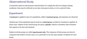
• Observational Study: The researcher observes and measures characteristics of a sample but does not change existing conditions. Data may be collected at one time, from past records, or over a period of time.

• Experiment: A treatment is applied to part of a population (treatment group), and responses are observed. A control group may receive a placebo (a harmless, fake treatment). Subjects in both groups are called experimental units. Comparing responses helps determine the effect of the treatment.

Methods of Data Collection

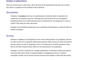
• Simulation: Uses mathematical or physical models to reproduce conditions of a situation or process. Useful for situations that are impractical or dangerous to create in real life. Example: An automobile manufacturer uses simulations with dummies to study crash effects.

• Survey: An investigation of one or more characteristics of a population, often by asking questions. Surveys can be conducted via interviews, internet, phone, or mail. Example: A survey of physicians to determine their preferred treatment methods.

Describing Data with Tables and Graphs

Frequency Distribution Construction

To organize raw data, a frequency distribution is constructed by following these steps:

1. List all raw data values.

2. Find the minimum and maximum values to compute the range: $Range = max - min$

3. Choose the number of classes (typically 5–10).

4. Compute class width: $Width = \frac{Range}{\text{Number of classes}}$ (round up if necessary)

5. Create class limits for each class interval.

6. Tally and count frequencies for each class.

7. Compute midpoints: $Midpoint = \frac{\text{Lower limit} + \text{Upper limit}}{2}$

8. Compute relative frequencies: $\text{Relative frequency} = \frac{f}{n}$

9. Compute cumulative frequencies by adding frequencies sequentially.

10. For continuous data, compute class boundaries: Lower boundary = lower limit − 0.5, Upper boundary = upper limit + 0.5

Key Table Structure:

Class #	Lower limit	Upper limit	Frequency (f)	Midpoint	Relative freq	Cumulative freq	Boundaries
1	____	____	____	____	____	____	____ – ____
2	____	____	____	____	____	____	____ – ____
...	...	...	...	...	...	...	...

Key Definitions

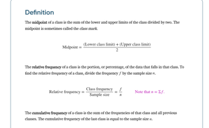
• Midpoint (Class Mark): $Midpoint = \frac{\text{Lower class limit} + \text{Upper class limit}}{2}$

• Relative Frequency: $\text{Relative frequency} = \frac{f}{n}$, where $f$ is class frequency and $n$ is sample size.

• Cumulative Frequency: The sum of the frequencies for that class and all previous classes.

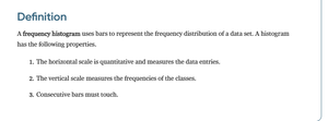
Frequency Histogram

A frequency histogram uses bars to represent the frequency distribution of a data set. Properties:

• The horizontal scale is quantitative and measures data entries.

• The vertical scale measures class frequencies.

• Consecutive bars must touch.

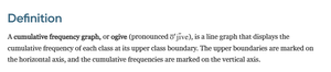
Cumulative Frequency Graph (Ogive)

An ogive is a line graph displaying the cumulative frequency of each class at its upper class boundary. The horizontal axis marks upper boundaries, and the vertical axis marks cumulative frequencies.

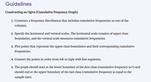
Constructing an Ogive

1. Construct a frequency distribution with cumulative frequencies.

2. Specify horizontal (upper class boundaries) and vertical (cumulative frequencies) scales.

3. Plot points for each upper class boundary and corresponding cumulative frequency.

4. Connect points with line segments.

5. Start at the lower boundary of the first class (cumulative frequency = 0) and end at the upper boundary of the last class (cumulative frequency = sample size).

Describing Data Numerically

Measures of Central Tendency

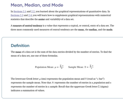
Measures of central tendency describe the center of a data set. The most common are the mean, median, and mode.

• Mean: The sum of all data entries divided by the number of entries. Population Mean: $\mu = \frac{\Sigma x}{N}$ Sample Mean: $\bar{x} = \frac{\Sigma x}{n}$

Weighted Mean

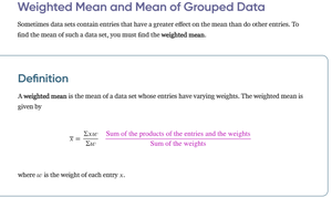
For data sets where entries have varying weights, the weighted mean is used:

• $\bar{x}_{\text{w}} = \frac{\Sigma xw}{\Sigma w}$, where $x$ is the value and $w$ is its weight.

Measures of Variation

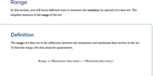
Variation describes the spread of data. The simplest measure is the range:

• $Range = \text{Maximum data entry} - \text{Minimum data entry}$

Quantitative Data

Quantitative data is measurable or countable, such as height, weight, salary, age, and time. Each value represents a quantity.

Variance and Standard Deviation

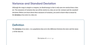
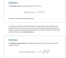
Variance and standard deviation are measures of how much data values deviate from the mean.

• Deviation: $x - \mu$ (for population data)

• Population Variance: $\sigma^2 = \frac{\Sigma (x - \mu)^2}{N}$

• Population Standard Deviation: $\sigma = \sqrt{\frac{\Sigma (x - \mu)^2}{N}}$

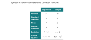
Symbols in Variance and Standard Deviation Formulas

Measure	Population	Sample
Variance	$\sigma^2$	$s^2$
Standard deviation	$\sigma$	$s$
Mean	$\mu$	$\bar{x}$
Number of entries	$N$	$n$
Deviation	$x - \mu$	$x - \bar{x}$
Sum of squares	$\Sigma (x - \mu)^2$	$\Sigma (x - \bar{x})^2$

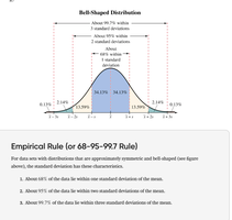
Empirical Rule (68-95-99.7 Rule)

For bell-shaped (normal) distributions:

• About 68% of data lie within one standard deviation of the mean.

• About 95% within two standard deviations.

• About 99.7% within three standard deviations.

Probability

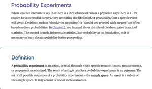
Probability Experiments

A probability experiment is an action or trial through which specific results (counts, measurements, or responses) are obtained. The result of a single trial is an outcome. The set of all possible outcomes is the sample space. An event is a subset of the sample space.

Identifying the Sample Space

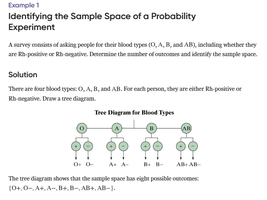
Example: A survey asks people for their blood types (O, A, B, AB) and Rh factor (positive or negative). The sample space consists of all possible combinations, shown in a tree diagram:

• Possible outcomes: O+, O−, A+, A−, B+, B−, AB+, AB−