Introductory Statistics Review: Data Types, Distributions, and Descriptive Statistics

Q1. What is the difference between numeric (quantitative) and categorical data? Give some examples of each.

Background

Topic: Types of Data

This question tests your understanding of the two main types of data in statistics: numeric (quantitative) and categorical (qualitative). Recognizing the difference is foundational for choosing appropriate statistical methods.

Key Terms:

• Numeric (Quantitative) Data: Data that represent measurable quantities and have meaningful numerical values (e.g., height, weight, test scores).

• Categorical (Qualitative) Data: Data that represent categories or groups (e.g., gender, color, type of car).

Step-by-Step Guidance

1. Define numeric (quantitative) data and think of examples where measurements or counts are involved.

2. Define categorical (qualitative) data and consider examples where data are sorted into groups or categories.

3. Be careful: Some variables may use numbers as labels (like area codes), but are not truly quantitative.

4. List at least two examples for each type of data.

Try solving on your own before revealing the answer!

Final Answer:

Numeric (Quantitative) Data: Data that can be measured or counted, such as height (in inches), weight (in pounds), or test scores (out of 100). Examples: Height of students, number of books, temperature.

Categorical (Qualitative) Data: Data that can be sorted into categories but not measured. Examples: Eye color, type of car, area code.

Remember, just because a variable uses numbers (like a jersey number or area code) doesn't mean it's quantitative.

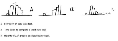
Q2. Match the variable name with the histogram by considering the likely shape of the distribution.

Background

Topic: Interpreting Histograms and Variable Types

This question asks you to use your understanding of data distributions to match real-world variables to their likely histogram shapes.

Key Terms:

• Histogram: A graphical representation of the distribution of numerical data.

• Distribution Shape: The general form of the data (e.g., symmetric, skewed right, skewed left).

Step-by-Step Guidance

1. Read the three variable descriptions: (1) Scores on an easy stats test, (2) Time taken to complete a short stats test, (3) Heights of 12th graders at a local high school.

2. Examine the shapes of the three histograms (A, B, C). Note which are symmetric, skewed right, or have other features.

3. Recall typical distributions for each variable: Test scores on an easy test often cluster at the high end (left-skewed), time to complete a test is often right-skewed, and heights are usually symmetric and bell-shaped.

4. Match each variable to the histogram shape that best fits its expected distribution.

Try solving on your own before revealing the answer!

Final Answer:

1. Scores on an easy stats test: Histogram C (left-skewed, most students score high). 2. Time taken to complete a short stats test: Histogram B (right-skewed, most finish quickly, a few take longer). 3. Heights of 12th graders: Histogram A (symmetric, bell-shaped).

Matching is based on typical real-world distributions for these variables.

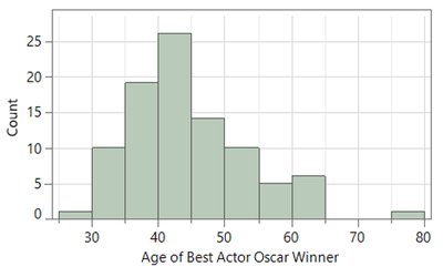
Q3. This histogram shows the distribution of the ages of 92 Best Actor Oscar winners (1929–2019). 1. How many Best Actor winners were between 50 and 60? 2. How old are the oldest winners? 3. What has been the most frequent age range of winners?

Background

Topic: Interpreting Histograms

This question tests your ability to read and interpret information from a histogram, including counts in intervals, identifying maximum values, and determining the mode (most frequent range).

Key Terms:

• Histogram: A bar graph showing the frequency of data within certain intervals (bins).

• Mode: The interval with the highest frequency (tallest bar).

Step-by-Step Guidance

1. Look at the histogram and identify the bar(s) that represent ages between 50 and 60. Count the height of these bars to estimate the number of winners in this range.

2. Find the rightmost bar(s) to determine the oldest age(s) of winners. Note the upper boundary of the last bar with nonzero height.

3. Identify the tallest bar in the histogram to determine the most frequent age range (the mode).

4. Write down the counts and age ranges you observe, but do not sum or finalize the answers yet.

Try solving on your own before revealing the answer!

Final Answer:

1. There are about 10 winners between 50 and 60 years old (sum the heights of the bars in that range). 2. The oldest winners are around 75–80 years old (rightmost bar). 3. The most frequent age range is 40–45 years (tallest bar).

These answers are based on reading the histogram's bar heights and age intervals.

Q4. If the data is skewed right, which is bigger: the mean or the median? If the data is skewed left, which is bigger: the mean or the median? What if it is symmetric?

Background

Topic: Measures of Center and Skewness

This question tests your understanding of how the mean and median relate to the shape of a data distribution (skewness).

Key Terms:

• Mean: The arithmetic average of the data.

• Median: The middle value when data are ordered.

• Skewness: The direction in which a distribution stretches (right = positive, left = negative).

Step-by-Step Guidance

1. Recall that in a right-skewed distribution, the tail is longer on the right (higher values).

2. Think about how extreme values (outliers) affect the mean and median. The mean is more sensitive to outliers than the median.

3. Apply this reasoning to left-skewed and symmetric distributions.

4. Summarize the relationship between mean and median for each case, but do not state the final comparison yet.

Try solving on your own before revealing the answer!

Final Answer:

In a right-skewed distribution, the mean is greater than the median. In a left-skewed distribution, the mean is less than the median. If the distribution is symmetric, the mean and median are approximately equal.

This is because the mean is pulled in the direction of the skew (toward the tail).

Q5. Suppose the heights of a sample of 200 men is recorded. The data is bell-shaped with an average of 68 inches and a standard deviation of 2.5 inches. Use the Empirical Rule to provide a rough sketch of the distribution.

Background

Topic: Empirical Rule (68-95-99.7 Rule)

This question tests your ability to apply the Empirical Rule to a normal (bell-shaped) distribution to estimate the spread of data.

Key Terms and Formula:

• Empirical Rule: In a normal distribution:

  • About 68% of data falls within 1 standard deviation of the mean.

  • About 95% within 2 standard deviations.

  • About 99.7% within 3 standard deviations.

• Mean ($\mu$): $68$ inches

• Standard Deviation ($\sigma$): $2.5$ inches

Step-by-Step Guidance

1. Identify the mean ($\mu = 68$) and standard deviation ($\sigma = 2.5$).

2. Calculate the intervals for 1, 2, and 3 standard deviations from the mean:

   • 1 SD: $\mu \pm \sigma$

   • 2 SD: $\mu \pm 2\sigma$

   • 3 SD: $\mu \pm 3\sigma$

3. Determine the percentage of data expected in each interval using the Empirical Rule.

4. Sketch or describe the bell-shaped curve, labeling the mean and the calculated intervals, but do not draw or finalize the sketch yet.

Try solving on your own before revealing the answer!

Final Answer:

1 SD: 68 ± 2.5 = 65.5 to 70.5 inches (about 68% of men) 2 SD: 68 ± 5 = 63 to 73 inches (about 95% of men) 3 SD: 68 ± 7.5 = 60.5 to 75.5 inches (about 99.7% of men)

The Empirical Rule tells us most heights fall within these ranges in a bell-shaped distribution.

Q6. Suppose the heights of a sample of 200 men are recorded. The data is bell-shaped with an average of 68 inches and a standard deviation of 2.5 inches. Find and interpret the z-score for a 72 inch tall man. Would you consider a 74 inch tall man to be unusual relative to the other men in this data set? Explain using the z-score.

Background

Topic: Z-scores and Standardization

This question tests your ability to calculate and interpret z-scores, which measure how many standard deviations a value is from the mean.

Key Formula:

$z = \frac{x - \mu}{\sigma}$

• $x$ = observed value

• $\mu$ = mean

• $\sigma$ = standard deviation

Step-by-Step Guidance

1. Identify the mean ($\mu = 68$), standard deviation ($\sigma = 2.5$), and the observed values ($x = 72$ and $x = 74$).

2. Plug $x = 72$ into the z-score formula to find the z-score for a 72 inch tall man.

3. Plug $x = 74$ into the z-score formula to find the z-score for a 74 inch tall man.

4. Recall that a z-score above 2 or below -2 is often considered unusual in a normal distribution. Use this to interpret whether 74 inches is unusual, but do not state the final conclusion yet.

Try solving on your own before revealing the answer!

Final Answer:

For 72 inches: $z = \frac{72 - 68}{2.5} = 1.6$ For 74 inches: $z = \frac{74 - 68}{2.5} = 2.4$

A z-score of 2.4 is greater than 2, so a 74 inch tall man would be considered somewhat unusual in this data set.

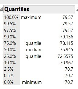
Q7. Find the 5 number summary and the Interquartile Range (IQR) using the JMP output.

Background

Topic: Five Number Summary and IQR

This question tests your ability to extract and interpret the five number summary and IQR from statistical software output.

Key Terms:

• Five Number Summary: Minimum, Q1 (first quartile), Median, Q3 (third quartile), Maximum.

• Interquartile Range (IQR): $IQR = Q3 - Q1$

Step-by-Step Guidance

1. Locate the minimum, Q1 (25% quartile), median (50%), Q3 (75% quartile), and maximum in the JMP output.

2. Write down each value as shown in the output.

3. Calculate the IQR by subtracting Q1 from Q3.

4. List the five number summary and the IQR, but do not finalize the calculation yet.

Try solving on your own before revealing the answer!

Final Answer:

Five number summary: Minimum = 70.7, Q1 = 72.5575, Median = 75.945, Q3 = 78.115, Maximum = 79.57 IQR = 78.115 - 72.5575 = 5.5575

The five number summary and IQR describe the spread and center of the data.

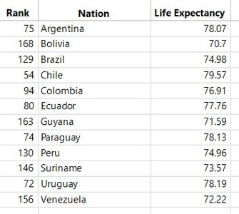
Q8. Repeat the preceding exercise by hand. You’ll notice that you get different answers than JMP which uses a somewhat more complicated method than just averaging the two numbers when there is an even number of observations.

Background

Topic: Calculating Five Number Summary and IQR by Hand

This question asks you to manually compute the five number summary and IQR from a data set, noting that software may use more complex algorithms for quartiles.

Key Terms:

• Five Number Summary: Minimum, Q1, Median, Q3, Maximum.

• Interquartile Range (IQR): $IQR = Q3 - Q1$

Step-by-Step Guidance

1. Order the data from smallest to largest.

2. Identify the minimum and maximum values.

3. Find the median (middle value).

4. Find Q1 (median of the lower half) and Q3 (median of the upper half).

5. Calculate the IQR as Q3 minus Q1, but do not finalize the values yet.

Try solving on your own before revealing the answer!

Final Answer:

Five number summary (by hand, using the data): Minimum = 70.7, Q1 = 73.57, Median = 75.945, Q3 = 78.13, Maximum = 79.57 IQR = 78.13 - 73.57 = 4.56

Manual calculation may differ slightly from software due to different methods for finding quartiles.

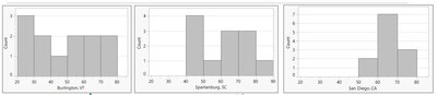
Q9. Order the following data sets by the size of the standard deviation.

Background

Topic: Standard Deviation and Spread

This question tests your ability to visually compare the spread of different data sets and order them by their standard deviation.

Key Terms:

• Standard Deviation: A measure of how spread out the values in a data set are around the mean.

Step-by-Step Guidance

1. Examine each histogram and note the spread of the data (how wide the bars are distributed).

2. Recall that a wider spread means a larger standard deviation.

3. Order the data sets from smallest to largest spread based on the histograms.

4. List the order, but do not finalize the answer yet.

Try solving on your own before revealing the answer!

Final Answer:

Order from smallest to largest standard deviation: San Diego, CA (narrowest), Burlington, VT (medium), Spartanburg, SC (widest).

Standard deviation increases as the spread of the data increases.

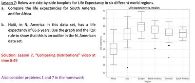
Q10. Below are side-by-side boxplots for Life Expectancy in six different world regions. a. Compare the life expectancies for South America and for Africa. b. Haiti, in N. America in this data set, has a life expectancy of 65.6 years. Use the graph and the IQR rule to show that this is an outlier in the N. American data set.

Background

Topic: Boxplots, Comparing Distributions, and Outliers

This question tests your ability to interpret boxplots, compare distributions, and use the IQR rule to identify outliers.

Key Terms and Formula:

• Boxplot: A graphical summary of the five number summary.

• IQR Rule for Outliers: A value is an outlier if it is below $Q1 - 1.5 \times IQR$ or above $Q3 + 1.5 \times IQR$.

Step-by-Step Guidance

1. Compare the medians, IQRs, and ranges for South America and Africa using the boxplots.

2. For part b, find the Q1, Q3, and IQR for North America from the boxplot or data.

3. Calculate the lower bound for outliers: $Q1 - 1.5 \times IQR$.

4. Check if Haiti's life expectancy (65.6 years) is below this lower bound, but do not finalize the calculation yet.

Try solving on your own before revealing the answer!

Final Answer:

a. South America has a higher median and less spread in life expectancy compared to Africa, which has a lower median and more variability. b. If Q1 for North America is about 75 and IQR is about 5, then the lower bound is 75 - 1.5*5 = 67.5. Haiti's life expectancy (65.6) is below this, so it is an outlier.

The IQR rule confirms Haiti is an outlier in the North American data set.