Introductory Statistics: Structured Study Notes (Chapters 1–3)

Statistics: Introduction and Data Collection

Definition and Key Concepts

Statistics is the science of collecting, organizing, summarizing, and analyzing data to answer questions or draw conclusions. Two major concepts in statistics are variation (differences or changes in an item) and data (observations gathered to draw conclusions). Measurements refer to numerical values, such as the number of customers.

• Data analysis: The process of examining and collecting data.

• Population: The complete set of people or objects being studied.

• Sample: A subset of the population from which data is obtained; should represent the population.

The Six W's of Data Collection

Surveys and experiments require understanding the following:

• Who: Individuals surveyed (respondents, subjects, participants, experimental units, records).

• What: What is being measured.

• When: When the research was conducted.

• Where: Where the research was conducted.

• Why: Purpose of the survey or experiment.

• How: How the survey or experiment was conducted.

Variables and Types of Data

• Variables: Characteristics recorded in a study.

• Numerical (Quantitative) Data: Represents measurable quantities (e.g., height, weight).

• Categorical Data: Describes qualities or categories (e.g., gender, color).

Data Formats

• Stacked Data: Spreadsheet format; each row is an individual, each column is a variable.

• Unstacked Data: Each column represents a variable from a different group; stores only two variables.

Frequency Tables

A frequency table displays each distinct outcome and its frequency. A relative frequency table shows percentages instead of counts.

Category	Count	Relative Frequency (%)
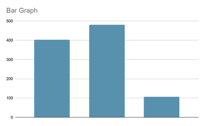
Rich	403	40.7
Middle	480	48.5
Poor	107	10.8

To calculate relative frequency: divide each count by the total, then multiply by 100.

Bar Graphs

Bar graphs visually display the frequency of each category. The height of each bar represents the count for its category.

Two-Way Tables

Two-way tables show the distribution of individuals along two categorical variables, displaying their relationships.

Types of Studies

• Controlled Experiment: Researchers assign subjects to groups; can establish cause-and-effect.

• Observational Study: Uses pre-existing groups; researchers do not assign subjects.

• Blind Study: Participants do not know their group assignment.

• Double Blind Study: Both participants and researchers do not know group assignments.

Describing Data with Tables and Graphs

Distribution and Frequency Tables

The distribution of a sample organizes data by values and their frequencies. Frequency tables and relative frequency tables are used to summarize this information.

Bar Charts and Pareto Charts

• Bar Chart: Displays frequency or relative frequency of categories; bars are separated.

• Pareto Chart: Bar chart with categories ordered from largest to smallest frequency.

Pie Charts

Pie charts represent categorical data as slices of a circle, with each slice proportional to the relative frequency.

Histograms

• Histogram: Displays quantitative data; bins represent ranges of values, and bars touch.

• Relative Frequency Histogram: Uses percentages instead of counts.

• Bin width affects detail; choose width to best show important features.

Dotplots

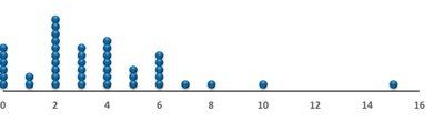
Dotplots are useful for small data sets with repeated values. Each dot represents a data point.

Stemplots (Stem-and-Leaf Plots)

• Divide each observation into a stem (all digits but the last) and a leaf (last digit).

• Useful for visualizing the shape and spread of data.

Distribution Shape, Center, and Spread

• Shape: Symmetric, skewed left, skewed right, unimodal, bimodal, multimodal.

• Outlier: Value much smaller or larger than the rest; may indicate error or genuine variation.

• Variability: Describes how spread out the data values are.

Describing Data Numerically

Measures of Center

• Mean: The average; sum of values divided by the number of values. Sensitive to outliers and skewed distributions.

• Median: The middle value; resistant to outliers.

Measures of Spread

• Variance: Average squared deviation from the mean; uses $s^2$.

• Standard Deviation: Square root of variance; measures typical distance from the mean. Uses $s$.

• Range: Difference between maximum and minimum values.

Quartiles and Interquartile Range (IQR)

• Quartiles: Divide data into four equal parts. Q1 (first quartile), Q2 (median), Q3 (third quartile).

• IQR: $IQR = Q3 - Q1$; measures spread of the middle 50% of data.

Z-Score

The z-score measures the distance of a value from the mean in standard deviations. It is calculated as:

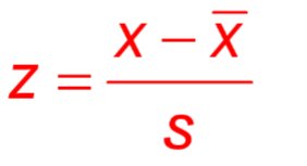
• A positive z-score: value above the mean.

• A negative z-score: value below the mean.

• Small z-score: value close to the mean.

• Large z-score: value far from the mean.

Example: Comparing Heights Using Z-Scores

• Mean height for men: 69.4 inches, standard deviation: 3.1 inches.

• Mean height for women: 63.8 inches, standard deviation: 2.8 inches.

• Man (73 inches): $z = \frac{73 - 69.4}{3.1} = 1.1$

• Woman (68 inches): $z = \frac{68 - 63.8}{2.8} = 1.5$

• The woman is taller relative to her gender.

The Empirical Rule (Bell-Shaped Distributions)

• About 68% of data falls within 1 standard deviation of the mean.

• About 95% within 2 standard deviations.

• About 99.7% within 3 standard deviations.

Additional info: These notes cover foundational concepts in statistics, including data collection, graphical and numerical summaries, and interpretation of data distributions. The included images directly illustrate bar graphs, dotplots, and the z-score formula, reinforcing the explanations provided.