Introductory Statistics: Structured Study Notes (Chapters 1–3)

Introduction to Statistics

Statistical and Critical Thinking

Statistics is the science of planning studies and experiments, obtaining data, and organizing, summarizing, presenting, analyzing, and interpreting those data to draw conclusions. Critical thinking is essential in evaluating the validity and reliability of statistical results.

• Statistics: The process of collecting, analyzing, and interpreting data.

• Data: Collections of observations, such as measurements, genders, or survey responses.

• Population: The complete collection of all measurements or data being considered.

• Census: Data collected from every member of the population.

• Sample: A subcollection of members selected from a population.

• Survey: Data collected from every member of a sample.

Example:

• Acme Corporation has 49 employees. Surveying 20 employees, 10% were left-handed. Population: All 49 employees. Sample: The 20 surveyed employees.

• 400 randomly selected adults surveyed for mean income. Population: All adults. Sample: The 400 surveyed adults.

Biased Samples and Sampling Methods

A sample is biased if it does not accurately represent the population. Voluntary-response samples (e.g., internet polls, mail-in polls) are often biased. The source of data can also introduce bias if it has a vested interest in the outcome.

• Statistical Significance: Results are statistically significant if they are unlikely to occur by chance (typically less than 5% probability).

• Practical Significance: Results are practically significant if they are important in real-world terms.

Types of Data

Parameters and Statistics

A parameter is a numerical measurement describing a characteristic of a population, while a statistic describes a characteristic of a sample.

• Quantitative Data: Numbers representing counts or measurements.

• Categorical Data: Names or labels; numbers used as designations (e.g., Social Security Numbers).

Types of Quantitative Data

• Discrete Data: Countable values (e.g., number of apples purchased).

• Continuous Data: Measurable values with infinite possibilities (e.g., amount of soda in cans).

Levels of Measurement

• Nominal: Names, labels, or categories only; cannot be ordered.

• Ordinal: Can be ordered, but differences are not meaningful.

• Interval: Ordered, meaningful differences, no natural zero.

• Ratio: Ordered, meaningful differences, natural zero.

Example:

• Brands of cat food: Nominal

• Battery life (hours): Ratio

• Temperatures (°F): Interval

• Socioeconomic status: Ordinal

Collecting Sample Data

Experiments and Observational Studies

Experiments involve applying treatments and observing effects, often using control and experimental groups. Observational studies involve measuring characteristics without intervention.

• Replication: Repeating an experiment on multiple individuals.

• Blinding: Subjects do not know if they receive treatment or placebo; double-blind if both subject and experimenter are unaware.

• Randomness: Assigning individuals to groups randomly.

Sampling Methods

• Simple Random Sampling: Every possible sample of size n has the same chance of being chosen.

• Systematic Sampling: Select every kth individual after a random start.

• Cluster Sampling: Divide population into clusters, randomly select clusters, and include all members from selected clusters.

• Stratified Sampling: Divide population into subgroups (strata) and sample from each subgroup.

• Convenience Sampling: Use data that are easy to obtain; often biased.

Random Number Generation Example:

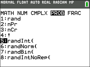
To generate random numbers on a TI-83/84 calculator:

• Press the MATH key.

• Navigate to the PROB menu.

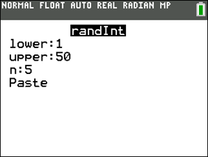
• Select 5:randInt( or 8:randIntNoRep(.

• Set lower limit, upper limit, and n (number of values).

• Press ENTER to generate random numbers.

Exploring Data with Tables and Graphs

Frequency Distributions

A frequency distribution (or frequency table) partitions data among categories or classes, listing each category with the number (frequency) of data values in it.

• Lower class limits: Smallest numbers in each class.

• Upper class limits: Largest numbers in each class.

• Class boundaries: Numbers separating classes without gaps.

• Class midpoints: Average of lower and upper class limits.

• Class width: Difference between consecutive lower class limits.

Entering and Sorting Data in a Calculator

To enter and sort data in a graphing calculator:

• Press STAT, choose 1:Edit, enter values in L1.

• To sort, press STAT, choose 2:SortA(, select L1, and press ENTER.

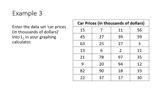
Example Data Table:

Car Prices (in thousands of dollars)
15, 7, 11, 56
45, 27, 39, 59
63, 25, 27, 3
13, 6, 2, 11
21, 78, 97, 35
9, 20, 94, 12
82, 90, 18, 33
22, 37, 17, 30

Histograms and Graphs

Histograms

A histogram is a graph with bars of equal width adjacent to each other, representing classes of quantitative data values (horizontal axis) and frequencies (vertical axis).

• Relative Frequency Histogram: Uses percentages or proportions instead of frequencies.

• Common Shapes: Bell-shaped, uniform, skewed right, skewed left.

Dotplots and Stemplots

• Dotplot: Each data value is plotted as a dot above a horizontal scale.

• Stemplot: Separates each value into a stem and leaf, showing distribution and retaining original values.

Scatterplots, Correlation, and Regression

Bivariate Data Sets and Correlation

Bivariate data sets involve two variables. Correlation exists when values of one variable are associated with values of another. Linear correlation is when the relationship can be approximated by a straight line.

• Linear Correlation Coefficient (r): Measures strength of linear relationship; ranges from -1 to 1.

• Positive Correlation: r close to 1; both variables increase together.

• Negative Correlation: r close to -1; one variable increases as the other decreases.

• No Correlation: r not close to -1 or 1.

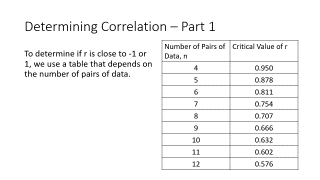
Critical Values Table:

Number of Pairs of Data, n	Critical Value of r
4	0.950
5	0.878
6	0.811
7	0.754
8	0.707
9	0.666
10	0.632
11	0.602
12	0.576

Describing, Exploring, and Comparing Data

Measures of Center

Measures of center describe the middle of a data set. The main measures are mean, median, mode, and midrange.

• Mean: Average of all data values. $\text{Mean} = \frac{\sum x}{n}$

• Median: Middle value when data are ordered.

• Mode: Value(s) occurring most frequently.

• Midrange: Value halfway between maximum and minimum. $\text{Midrange} = \frac{\text{Max} + \text{Min}}{2}$

Calculating Measures with a Calculator

Enter data into L1, sort, and use calculator functions to find mean, median, mode, and midrange.

Estimating a Mean Using a Frequency Distribution

To estimate the mean from a frequency distribution:

• Find midpoints for each class.

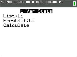
• Enter midpoints into L1 and frequencies into L2.

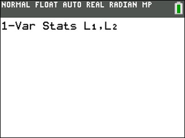
• Use 1-Var Stats with L1 and L2.

Measures of Variation

Range, Standard Deviation, and Variance

• Range: Difference between maximum and minimum values. $\text{Range} = \text{Max} - \text{Min}$

• Standard Deviation: Measures how much values deviate from the mean. $s = \sqrt{\frac{\sum (x - \bar{x})^2}{n-1}}$

• Variance: Square of the standard deviation. $s^2 = \frac{\sum (x - \bar{x})^2}{n-1}$

Empirical Rule

For bell-shaped distributions:

• 68% of values within 1 standard deviation of mean

• 95% within 2 standard deviations

• 99.7% within 3 standard deviations

Measures of Relative Standing and Boxplots

Z Scores

• Z Score: Indicates how many standard deviations a value is from the mean. $z = \frac{x - \mu}{\sigma}$

• Significantly low: z ≤ -2; significantly high: z ≥ 2

Percentiles and Quartiles

• Percentile: Indicates the percentage of values below a given value.

• Quartiles: Divide data into four equal parts.

• Five-Number Summary: Minimum, Q1, Median, Q3, Maximum

Boxplots

Boxplots graphically represent the five-number summary. Standard and modified boxplots can be created using a graphing calculator.