Inverse Normal Calculations in the Normal Distribution

Normal Probability Distributions

Inverse Normal Calculations

The inverse normal calculation is a method used to determine the value of a variable (x or z) that corresponds to a specified area (probability) under the normal curve. This is essential for solving problems where the probability is known, but the corresponding value is unknown.

• Definition: The inverse normal calculation finds the value of x or z given a probability (area) under the normal curve.

• Formula: The relationship between x and z is given by: $a = \mu + \sigma z$ where $\mu$ is the mean, $\sigma$ is the standard deviation, and $z$ is the z-score corresponding to the desired area.

• Sign of z-score:

  • If the value is below the mean, the z-score is negative.

  • If the value is above the mean, the z-score is positive.

• Steps for Inverse Normal Calculation:

  1. Draw a rough normal curve and label the mean.

  2. Determine the location of the desired value relative to the mean to find the sign of z.

  3. Use the z-table to find the z-score corresponding to the given area.

  4. Apply the formula $a = \mu + \sigma z$ to solve for the unknown value.

Examples of Inverse Normal Calculations

Several examples illustrate the application of inverse normal calculations:

• Example 1: Given population mean $\mu = 90$ and standard deviation $\sigma = 6$, find $a$ such that $P(x > a) = 0.95$.

  • Area to the right of $a$ is 0.95, so $a$ is to the left of the mean and z is negative.

  • From the z-table, $z = -1.645$ (since $P(z < 1.645) = 0.95$).

  • Apply the formula: $a = 90 + 6 \times (-1.645) = 80.13$.

• Example 2: If the mean is 500 and standard deviation is 100, find $x$ such that 60% of the area is to the left.

  • Area to the left of $a$ is 0.6, so z is positive.

  • From the z-table, $z = 0.25$ (since $P(z < 0.25) \approx 0.6$).

  • Apply the formula: $a = 500 + 100 \times 0.25 = 525$.

• Example 3: For Alzheimer’s disease data (mean age 80, standard deviation 16):

  • Find $a$ such that $P(x > a) = 0.9$:

    • From z-table, $z = -1.28$ (since $P(z > -1.28) = 0.9$).

    • $a = 80 + 16 \times (-1.28) = 59.52$.

  • Find $a$ such that $P(x < a) = 0.975$:

    • From z-table, $z = 1.96$ (since $P(z < 1.96) = 0.975$).

    • $a = 80 + 16 \times 1.96 = 111.36$.

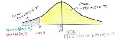
• Example 4: Lifespan of palm trees (mean 70, standard deviation 1.5):

  • Find $a$ such that $P(x < a) = 0.21$:

    • Area to the left is 0.21, so z is negative.

    • From z-table, $z \approx -0.81$ (since $P(z < -0.81) \approx 0.21$).

    • $a = 70 + 1.5 \times (-0.81) = 68.785$ (rounded to 68.8).

Using the Standard Normal Table (z-table)

The z-table is used to find the area under the standard normal curve corresponding to a given z-score. It is essential for inverse normal calculations.

• Purpose: To determine the probability (area) associated with a specific z-score.

• Application: Used in step 3 of the inverse normal calculation to find the z-score for a given area.

Z	.00	.01	.02	.03	.04	.05	.06	.07	.08	.09
0.0	.50000	.50399	.50798	.51197	.51595	.51994	.52392	.52790	.53188	.53586
0.1	.53983	.54380	.54776	.55172	.55567	.55962	.56356	.56749	.57142	.57535
0.2	.57926	.58317	.58706	.59095	.59483	.59871	.60257	.60642	.61026	.61409
0.3	.61791	.62172	.62552	.62930	.63307	.63683	.64058	.64431	.64803	.65173
0.4	.65542	.65910	.66276	.66640	.67003	.67364	.67724	.68082	.68439	.68793
0.5	.69146	.69497	.69847	.70194	.70540	.70884	.71226	.71566	.71904	.72240
0.6	.72575	.72907	.73237	.73565	.73891	.74215	.74537	.74857	.75175	.75490
0.7	.75804	.76115	.76424	.76730	.77035	.77337	.77637	.77935	.78230	.78524
0.8	.78814	.79103	.79389	.79673	.79955	.80234	.80511	.80785	.81057	.81327
0.9	.81594	.81859	.82121	.82381	.82639	.82894	.83147	.83398	.83646	.83891
1.0	.84134	.84375	.84614	.84849	.85083	.85314	.85543	.85769	.85993	.86214
1.1	.86433	.86650	.86864	.87076	.87286	.87493	.87698	.87900	.88100	.88298
1.2	.88493	.88686	.88877	.89065	.89251	.89435	.89617	.89796	.89973	.90147
1.3	.90320	.90490	.90658	.90824	.90988	.91149	.91309	.91466	.91621	.91774
1.4	.91924	.92073	.92220	.92364	.92507	.92647	.92785	.92922	.93056	.93189
1.5	.93319	.93448	.93574	.93699	.93822	.93943	.94062	.94179	.94294	.94408
1.6	.94520	.94630	.94738	.94845	.94950	.95053	.95154	.95254	.95352	.95449
1.7	.95543	.95637	.95729	.95819	.95907	.95994	.96080	.96164	.96246	.96327
1.8	.96407	.96485	.96562	.96638	.96712	.96784	.96856	.96926	.96995	.97062
1.9	.97128	.97193	.97257	.97320	.97381	.97441	.97500	.97558	.97615	.97670
2.0	.97725	.97778	.97831	.97882	.97932	.97982	.98030	.98077	.98124	.98169

Visual Representation of Inverse Normal Calculation

The following image illustrates the area under the normal curve for Example 4, showing the relationship between the mean, the value 'a', and the probability: