Least-Squares Regression and Coefficient of Determination: Study Notes

Least-Squares Regression and Coefficient of Determination

Least-Squares Regression Line

The least-squares regression line is a statistical method used to model the relationship between two quantitative variables. It minimizes the sum of the squared differences between observed values and the values predicted by the line.

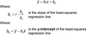
• Equation: The regression line is represented as $\hat{y} = b_1 x + b_0$.

• Slope ($b_1$): Indicates the change in the response variable for a one-unit increase in the explanatory variable.

• Y-intercept ($b_0$): Represents the predicted value of the response variable when the explanatory variable is zero.

• Calculation:

  • $b_1 = r \cdot \frac{S_y}{S_x}$, where $r$ is the correlation coefficient, $S_y$ is the standard deviation of the response variable, and $S_x$ is the standard deviation of the explanatory variable.

  • $b_0 = \overline{y} - b_1 \overline{x}$, where $\overline{y}$ and $\overline{x}$ are the means of the response and explanatory variables, respectively.

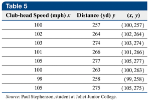
Example: Club-head Speed and Golf Ball Distance

Consider the relationship between club-head speed and the distance a golf ball travels. The data below represent eight swings, showing a linear relationship between speed and distance.

• Data Table:

Club-head Speed (mph) x	Distance (yd) y	(x, y)
100	257	(100, 257)
102	264	(102, 264)
103	274	(103, 274)
101	266	(101, 266)
105	277	(105, 277)
100	263	(100, 263)
99	258	(99, 258)
105	275	(105, 275)

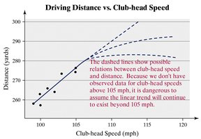
• Scatter Plot and Regression Line: Visualizing the data helps confirm the linear relationship.

• Prediction Example: Using the regression equation, one can predict the mean distance for a club-head speed of 103 mph.

Interpretation of Slope and Y-Intercept

Understanding the meaning of the slope and y-intercept is crucial for interpreting regression results in context.

• Slope: If club-head speed increases by 1 mph, the distance the golf ball travels increases by approximately 3.1661 yards, on average.

• Y-intercept: The y-intercept is the predicted distance when club-head speed is 0 mph. However, if 0 is not a reasonable value for the explanatory variable (e.g., a club-head speed of 0 mph), the y-intercept should not be interpreted.

• Extrapolation: Predictions should not be made for values outside the observed range (e.g., predicting distance for club-head speeds above 105 mph), as the linear relationship may not hold.

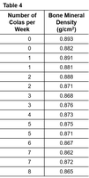
Case Study: Cola Consumption vs. Bone Mineral Density

Researchers investigated whether cola consumption is associated with lower bone mineral density in women. The data below show the number of colas consumed per week and bone mineral density for a sample of 15 women.

• Data Table:

Number of Colas per Week	Bone Mineral Density (g/cm2)
0	0.893
1	0.892
1	0.891
2	0.881
2	0.888
3	0.871
3	0.876
4	0.873
5	0.875
6	0.871
7	0.867
8	0.862
8	0.855

• Correlation: The correlation coefficient is $r = -0.806$, indicating a strong negative linear relationship.

• Regression Line: The least-squares regression line can be calculated using the formulas above, treating cola consumption as the explanatory variable.

• Interpretation:

  • Slope: Represents the change in bone mineral density for each additional cola consumed per week.

  • Y-intercept: Represents the predicted bone mineral density when cola consumption is zero, provided this is a reasonable value.

• Prediction Example: Predict the bone mineral density for a woman who consumes four colas per week and compare to observed values.

• Extrapolation Warning: Avoid using the model to predict bone mineral density for values outside the observed range (e.g., two colas per day).

Coefficient of Determination ($R^2$)

The coefficient of determination ($R^2$) quantifies the proportion of variation in the response variable explained by the regression model.

• Definition: $R^2$ ranges from 0 to 1. Higher values indicate a better fit.

• Interpretation:

  • $R^2 = 0$: The regression line explains none of the variation.

  • $R^2 = 1$: The regression line explains all the variation.

  • Intermediate values indicate partial explanatory power.

• Calculation: $R^2 = r^2$, where $r$ is the correlation coefficient.

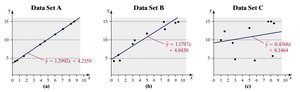
• Examples:

  • Data Set A: $R^2 = 99.99\%$ (almost all variability explained)

  • Data Set B: $R^2 = 94.7\%$ (most variability explained)

  • Data Set C: $R^2 = 9.4\%$ (very little variability explained)

• Application: For the club-head speed vs. distance data, and the cola consumption vs. bone mineral density case study, $R^2$ can be computed and interpreted to assess the strength of the linear relationship.

Summary Table: Regression Concepts

Concept	Definition	Formula
Regression Line	Best-fit line for linear relationship	$\hat{y} = b_1 x + b_0$
Slope ($b_1$)	Change in y per unit change in x	$b_1 = r \cdot \frac{S_y}{S_x}$
Y-intercept ($b_0$)	Predicted y when x = 0	$b_0 = \overline{y} - b_1 \overline{x}$
Coefficient of Determination ($R^2$)	Proportion of variance explained	$R^2 = r^2$

Additional info: These notes expand on the original content by providing definitions, formulas, examples, and warnings about extrapolation, making them suitable for exam preparation in a statistics course.