Least Squares Regression, Residuals, and Model Selection in Statistics

Least Squares Regression and Model Selection

Statistical Notation and Regression Models

Regression models are fundamental tools in statistics for examining relationships between variables and making predictions. The process involves fitting a line to data points to best represent the relationship between an explanatory variable (x) and a response variable (y).

• Simple Linear Regression: Models the relationship between two quantitative variables using a straight line.

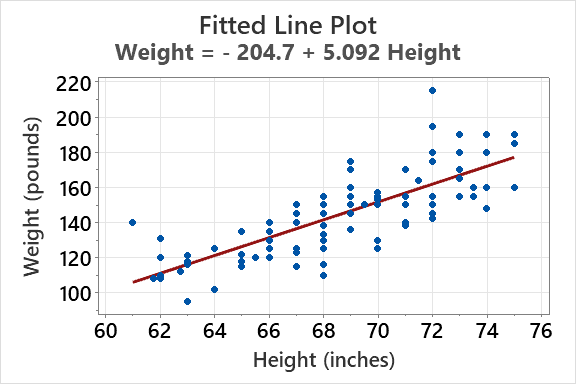
• Fitted Line Plot: Visualizes the regression line and the data points, helping to assess the fit.

• Residual Plot: Shows the differences between observed and predicted values, useful for diagnosing model fit.

• Storage of Residuals and Fits: Residuals and fitted values are often stored for further analysis.

• Prediction: Once a regression model is obtained, predictions for new values can be made.

Conditions for Descriptive Least Squares Regression

To ensure the validity of a least squares regression model, several conditions must be checked:

• Quantitative Variable Condition: Both variables must be quantitative.

• Straight Line Condition: The scatterplot should indicate a linear relationship. Residual plots should also reflect this pattern.

• No Outlier Condition: Outliers can dramatically influence the fit. If problematic, least squares regression should not be used.

• Equal Spread Condition: The spread of residuals should be consistent across all values of x (no fanning).

Identifying Unusual Observations

Unusual observations can affect regression models in different ways:

• Large Outliers (R Flag): Observations with large standardized residuals (absolute value > 2.00) are flagged as R. These increase the standard error (se) and decrease R2.

• High Leverages (X Flag): Observations far from the mean of x (x-bar) are flagged as X. These can lead to imprecise predictions at those values.

• Highly Influential Observations: Observations that greatly change model coefficients when removed. They may have X or RX flags and can sometimes be hidden in residual plots.

Model Selection and R2

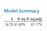
The coefficient of determination, R2, measures how well the regression line predicts the response variable. However, it does not indicate whether the best model has been selected. Meeting model conditions is essential for selecting the best model.

• R2: Indicates the proportion of variance in the response variable explained by the model.

• Adjusted R2: Adjusts for the number of predictors, providing a more accurate measure for model comparison.

Residuals and Standardized Residuals

Calculation of Standardized Residuals

Standardized residuals are used to identify unusual observations in regression analysis. They account for the leverage of each data point.

• Standardized Residual (Z): Measures how far an observation is from the regression line, standardized by its leverage.

• Leverage (hi): Indicates the influence of each observation on the fitted values.

Formula:

$Z = \frac{e_i}{s \sqrt{1 - h_i}}$

Where $e_i$ is the residual for observation $i$, $s$ is the standard error, and $h_i$ is the leverage.

Working with Summary Values

Original Observations vs. Summary Data

Regression analysis can be performed on both original data and summary values. Summary data often involves using averages or aggregated values, which can affect the interpretation and fit of the model.

• Original Data: Uses individual observations for regression analysis.

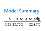
• Summary Data: Uses aggregated values (e.g., group means) for regression, which may reduce variability and increase R2.

• Comparison: Models fitted to summary data often show higher R2 and lower standard error due to reduced variability.

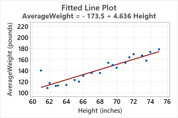
Example: Comparing fitted line plots and model summaries for original and summary data demonstrates the impact of aggregation on regression results.

Final Tips for Regression Analysis

• Always check model conditions before interpreting regression results.

• Use residual and leverage flags to identify and address unusual observations.

• Compare models using R2 and adjusted R2, but ensure conditions are met for valid model selection.

• Extraordinary cases and deviations from the model can provide valuable insights.

Additional info: The notes reference Minitab software for regression analysis, which is commonly used in statistics courses for generating fitted line plots, residual plots, and model summaries.