 Back
BackLinear Regression: Concepts, Computation, and Interpretation
Study Guide - Smart Notes
 Tailored notes based on your materials, expanded with key definitions, examples, and context.
Linear Regression
Introduction to Linear Regression
Linear regression is a statistical method used to model the relationship between a quantitative response variable and one or more explanatory variables. The simplest form, simple linear regression, involves one predictor and one response variable, aiming to find the best-fitting straight line through the data.
Scatterplots and the Linear Model
Visualizing Relationships: Scatterplots
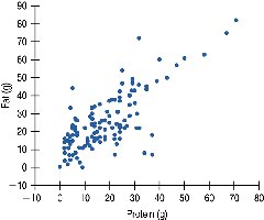
Scatterplots are essential for visualizing the relationship between two quantitative variables. Each point represents an observation, with the x-axis for the predictor and the y-axis for the response variable. Patterns in the scatterplot can suggest the form, direction, and strength of the relationship.
Direction: Indicates whether the relationship is positive or negative.
Form: Linear or nonlinear patterns.
Strength: How closely the points follow a clear form.
Unusual Features: Outliers or clusters that deviate from the main pattern.

The Linear Model
The linear model describes the relationship between variables using the equation:
Slope (b1): The change in the response variable for each unit increase in the predictor.
Intercept (b0): The expected value of the response when the predictor is zero.
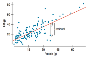
Least Squares: The Line of Best Fit
Finding the Best-Fitting Line
The best-fitting line in linear regression is the one that minimizes the sum of the squared residuals (vertical distances between observed and predicted values). This is known as the least squares line.
Residuals
A residual is the difference between an observed value and the value predicted by the regression line:
Residuals help assess the fit of the model.
Ideally, residuals should be randomly scattered around zero.
Conditions for Using Linear Regression
Regression Conditions
Before applying linear regression, several conditions must be checked:
Quantitative Variables Condition: Both variables must be quantitative.
Straight Enough Condition: The relationship should be approximately linear.
No Outliers Condition: There should be no influential outliers.
Does the Plot Thicken? Condition: The spread of residuals should be roughly constant across all values of x.
Interpreting Regression Coefficients
Understanding Slope and Intercept
The slope and intercept have specific interpretations in context:
Slope (b1): Represents the average change in the response variable for each one-unit increase in the predictor variable.
Intercept (b0): Represents the expected value of the response variable when the predictor is zero. Sometimes, the intercept may not have a meaningful interpretation in context.
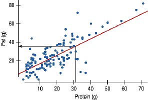
Example: For the Burger King data, if the slope is 0.91, then for every additional gram of protein, we expect an additional 0.91 grams of fat, on average.
Roles for Variables in Regression
Predictor and Response Variables
In regression, the explanatory (predictor) variable is plotted on the x-axis, and the response variable is plotted on the y-axis. The choice of which variable is which is critical, as regression is not symmetric with respect to x and y.
Predictor (x): The variable used to predict or explain changes in the response.
Response (y): The variable being predicted or explained.
Examining Residuals
Assessing Model Fit with Residuals
Residual plots are used to check the assumptions of linear regression. A good model will have residuals that are randomly scattered with no clear pattern.
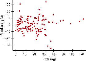
Example: The residuals for the Burger King menu regression appear randomly scattered, indicating a good fit.
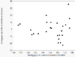
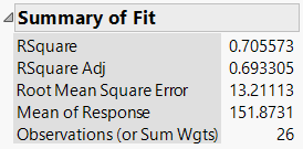
Residuals for Other Data Sets
Examining residuals for other data sets, such as mortgages versus interest rates, can reveal patterns or violations of regression assumptions.
R2: The Variation Accounted for by the Model
Understanding R2
R2 (the coefficient of determination) measures the proportion of the variance in the response variable that is explained by the regression model. It is calculated as the square of the correlation coefficient (r):
R2 = 0: The model explains none of the variance.
R2 = 1: The model explains all the variance.
Example: For the Burger King model, if r = 0.76, then R2 = 0.58, meaning 58% of the variance in fat content is explained by protein content.
Statistical Significance in Regression
Testing for Statistical Significance
To determine if the observed linear association is real or due to chance, we test the null hypothesis that the slope is zero. The p-value from the regression output indicates whether the association is statistically significant.
p-value < 0.05: The association is statistically significant.
p-value > 0.05: The association is likely due to random chance.
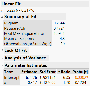
Example: Random Data and Regression
When analyzing data generated by random processes (e.g., two spinners), a regression may yield a nonzero slope by chance. The p-value helps determine if this is meaningful.


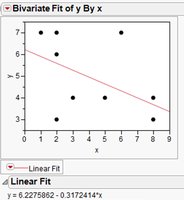
In this example, the p-value is 0.1284, which is greater than 0.05, indicating the regression is not statistically significant.
Summary Table: Regression Output Interpretation
Statistic | Interpretation |
|---|---|
Slope (b1) | Change in y for each unit increase in x |
Intercept (b0) | Expected value of y when x = 0 |
R2 | Proportion of variance in y explained by x |
p-value | Probability that the observed association is due to chance |
Precautions in Using Regression
Extrapolation
Do not use the regression equation to predict values outside the range of the original data. Extrapolation can lead to unreliable and inaccurate predictions.
Regression Assumptions and Review
Quantitative Variables Condition
Straight Enough Condition
No Outliers Condition
Does the Plot Thicken? Condition
Always check these conditions before interpreting or using a regression model.
