Linear Regression, Correlation, and Analysis of Variance in Statistics

Statistical Notation and Normal Distribution

Notation for Parameters and Statistics

Statistical notation is essential for distinguishing between population parameters and sample statistics. For the normal distribution, the notation y ~ N(\mu, \sigma) indicates that the variable y is normally distributed with mean \mu and standard deviation \sigma.

• Parameter: A value that describes a characteristic of a population (e.g., \mu, \sigma).

• Statistic: A value calculated from sample data (e.g., sample mean, sample standard deviation).

Graphs with Two Quantitative Variables

Scatterplots and Correlation

Scatterplots are used to visualize the relationship between two quantitative variables. Correlation quantifies the strength and direction of a linear relationship between variables.

• Scatterplot: Each point represents a pair of values for two variables.

• Correlation coefficient (r): Measures linear association; ranges from -1 to 1.

• Positive correlation: As one variable increases, the other tends to increase.

• Negative correlation: As one variable increases, the other tends to decrease.

Example: The correlation between MaxSpeed and CentralPressure is r = -0.951, indicating a strong negative linear relationship.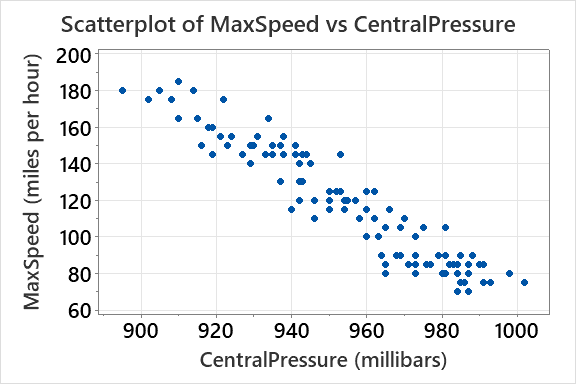

Regression and Linear Models

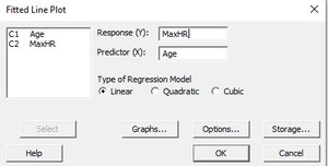
Simple Linear Regression

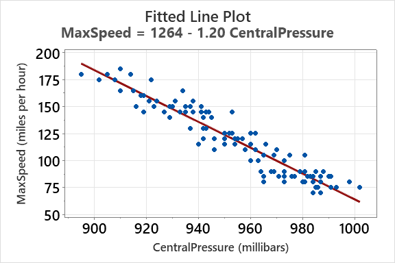
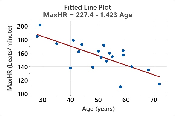
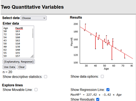
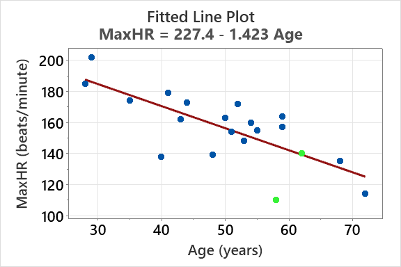
Regression analysis estimates the relationship between a response variable and a predictor variable. The fitted line plot shows the regression equation and the data points.

• Regression equation: $y = \beta_0 + \beta_1 x$

• Slope (\beta_1): Change in y for a one-unit increase in x.

• Intercept (\beta_0): Predicted value of y when x = 0 (may not always have a logical interpretation).

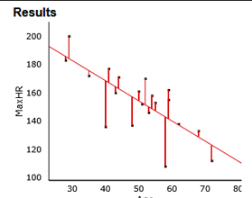
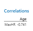
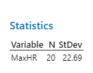
Example: For predicting MaxHR from Age: 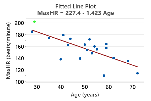$\text{MaxHR} = 227.4 - 1.423 \times \text{Age}$

Anscombe’s Quartet

Importance of Data Visualization

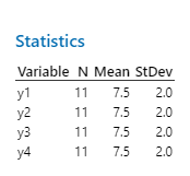
Anscombe’s Quartet consists of four datasets with nearly identical summary statistics but very different relationships when graphed. This demonstrates the importance of visualizing data before analysis.

• Non-resistant statistics: Statistics that can be heavily influenced by outliers or unusual data patterns.

• Graphical analysis: Reveals patterns, outliers, and relationships not evident in summary statistics.

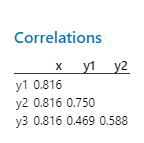
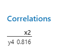
Example: All four datasets have similar means, standard deviations, and correlations, but their scatterplots are visually distinct.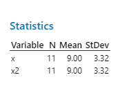

Examining Residuals

Definition and Calculation

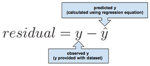
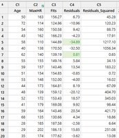
Residuals are the differences between observed values and predicted values from a regression model. They are used to assess model fit and identify outliers.

• Residual formula: $\text{residual} = y - \hat{y}$

• Interpretation: Positive residual: observed value is above the predicted value; negative residual: observed value is below the predicted value.

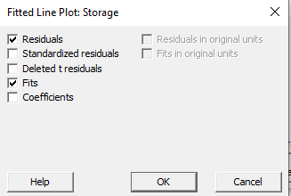
Visualization and Storage of Residuals

Residuals can be visualized on fitted line plots and stored for further analysis. Comparing residuals helps identify influential points and assess model assumptions.

• Largest residual: Indicates the observation farthest from the regression line.

• Smallest residual: Indicates the observation closest to the regression line.

Ordinary Least Squares (OLS) Regression

Least Squares Criterion

OLS regression estimates coefficients by minimizing the sum of squared residuals. This method ensures the best linear fit to the data.

• Sum of squared residuals: $\sum (y_i - \hat{y}_i)^2$

• Least squares criterion: Minimizes the total squared error between observed and predicted values.

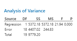
Analysis of Variance (ANOVA) in Regression

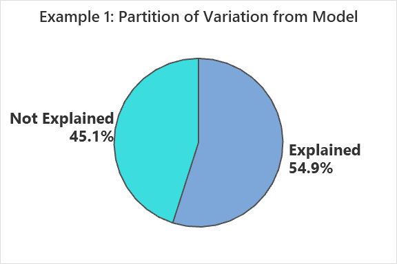
Partitioning Variation

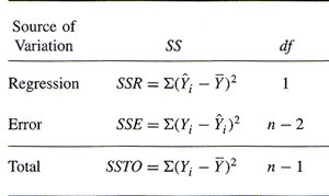
ANOVA tables partition the total variation in the response variable into variation explained by the model and variation due to error (residuals).

• Total Sum of Squares (SSTO): $\sum (Y_i - \overline{Y})^2$

• Regression Sum of Squares (SSR): $\sum (\hat{Y}_i - \overline{Y})^2$

• Error Sum of Squares (SSE): $\sum (Y_i - \hat{Y}_i)^2$

R Squared (Coefficient of Determination)

Interpretation and Calculation

R squared (R2) measures the proportion of variance in the response variable explained by the model. It is calculated as the squared correlation coefficient.

• Formula: $R^2 = \frac{\text{SSR}}{\text{SSTO}}$

• Interpretation: Higher R2 indicates a more useful model for prediction.

• Range: 0 to 1 (or 0% to 100%)

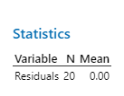
Standard Deviation of Residuals (se) and Model Evaluation

Comparing se and sy

The standard deviation of residuals (se) measures the average spread of residuals. Comparing se to the standard deviation of the response variable (sy) helps evaluate model effectiveness.

• se: Standard deviation of residuals; lower values indicate better model fit.

• sy: Standard deviation of the response variable.

• Interpretation: If se < sy, the model is useful for prediction.

Regression Assumptions and Conditions

Key Assumptions

For valid inference in linear regression, several assumptions must be met:

• Linearity: The relationship between predictor and response is linear.

• Independence: Observations are independent.

• Homoscedasticity: Constant variance of residuals across levels of predictor.

• Normality: Residuals are approximately normally distributed.

Summary Table: ANOVA Components

The ANOVA table summarizes the partitioning of variation in regression analysis.

Source of Variation	SS	df
Regression	SSR = $\sum (\hat{Y}_i - \overline{Y})^2$	1
Error	SSE = $\sum (Y_i - \hat{Y}_i)^2$	n - 2
Total	SSTO = $\sum (Y_i - \overline{Y})^2$	n - 1

Attributes of R Squared and se

Reporting and Interpretation

Always report both R2 and se when evaluating regression models. R2 is a descriptive measure, while se is reported in the original units of the response variable.

• R2: Indicates the fraction of variability explained by the model.

• se: Provides context for prediction accuracy.

Applications and Examples

Predicting Maximum Heart Rate

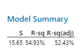
Regression models can be used to predict physiological variables such as maximum heart rate based on age or other predictors. The effectiveness of the model is evaluated using R2 and se.

• Example: $\text{MaxHR} = 227.4 - 1.423 \times \text{Age}$

• R2: 54.9% of the variation in MaxHR is explained by age.

• se: 15.65 beats/minute (standard deviation of residuals).

Anscombe’s Quartet Revisited

R2 Calculation

For all four graphs in Anscombe’s Quartet, the squared correlation coefficient is $R^2 = (0.816)^2 = 0.67$ or 67%.

• Interpretation: Despite identical R2 values, the data relationships are visually distinct, emphasizing the importance of graphing data.

Conclusion

Linear regression, correlation, and ANOVA are fundamental tools in statistics for analyzing relationships between quantitative variables. Visualizing data, examining residuals, and understanding model fit are essential for effective statistical analysis.