Linear Regression: Modeling, Residuals, and Interpretation

Linear Regression and Its Application

Introduction to Linear Regression

Linear regression is a statistical method used to model the relationship between two quantitative variables by fitting a straight line to the observed data. This line, called the regression line, allows us to predict the value of one variable (the response or dependent variable) based on the value of another (the explanatory or independent variable).

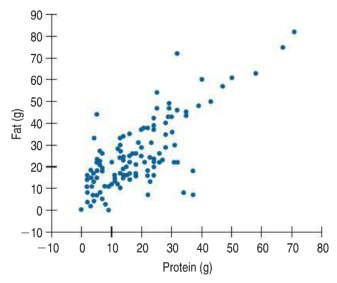
• Scatterplots are used to visualize the relationship between two quantitative variables.

• Correlation coefficient (r) measures the strength and direction of the linear relationship.

• A positive, linear, and moderately strong relationship is indicated by an r value close to +1.

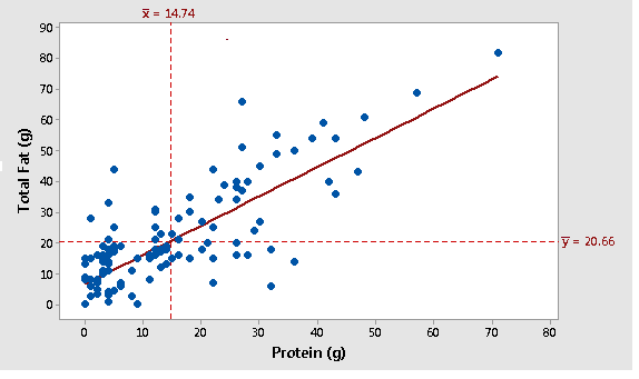
The Linear Regression Model

The linear regression model provides an equation for the best-fitting straight line through the data. This model is used for prediction and understanding the association between variables.

• The general form of the regression equation is: $\hat{y} = b_0 + b_1 x$

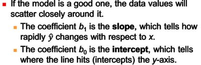
• Slope (b1): Indicates the expected change in y for a one-unit increase in x.

• Intercept (b0): The predicted value of y when x = 0.

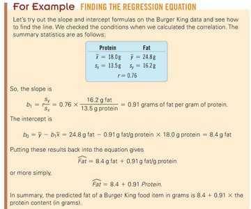
Finding the Regression Equation

To determine the regression equation, calculate the slope and intercept using summary statistics and the correlation coefficient.

• The slope is calculated as: $b_1 = r \frac{s_y}{s_x}$

• The intercept is calculated as: $b_0 = \bar{y} - b_1 \bar{x}$

• Where $r$ is the correlation coefficient, $s_y$ and $s_x$ are the standard deviations of y and x, and $\bar{y}$ and $\bar{x}$ are their means.

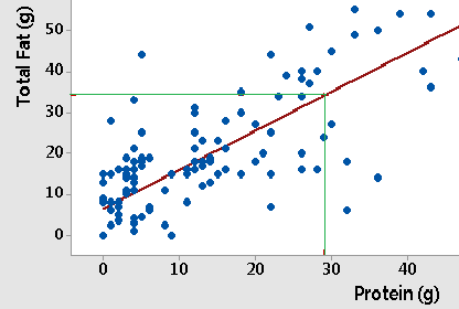
Making Predictions with the Regression Model

Once the regression equation is established, it can be used to predict the response variable for given values of the explanatory variable.

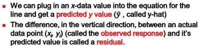
• Substitute the value of x into the regression equation to obtain the predicted y (denoted $\hat{y}$).

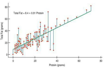
• Example: Predicting fat content for a Burger King item with 29g protein using $\hat{\text{Fat}} = 6.65 + 0.95 \times \text{Protein}$ yields $\hat{\text{Fat}} = 34.2$ grams.

Understanding and Analyzing Residuals

Definition and Calculation of Residuals

Residuals are the differences between observed values and the values predicted by the regression model. They measure the vertical distance from each data point to the regression line.

• Residual for the i-th observation: $e_i = y_i - \hat{y}_i$

• Positive residual: Actual value is greater than predicted (underestimate).

• Negative residual: Actual value is less than predicted (overestimate).

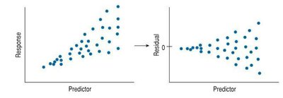
Visualizing Residuals

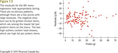
Plotting residuals helps assess the fit of the model and check for violations of regression assumptions.

• A good model will have residuals scattered randomly around zero, with no obvious patterns.

• Residual plots can reveal non-linearity, unequal variance, or outliers.

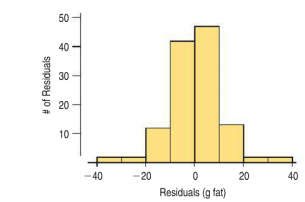
Distribution of Residuals

The distribution of residuals should be approximately normal (unimodal and symmetric) if the linear model is appropriate.

• Histogram and normal probability plots are used to assess normality.

• Most residuals should fall within two standard deviations of zero (68-95-99.7 rule).

Assessing Model Fit: R-Squared and Standard Deviation of Residuals

R-Squared (Coefficient of Determination)

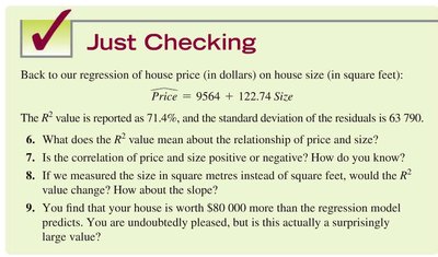
R-squared ($R^2$) measures the proportion of the variance in the response variable that is explained by the regression model.

• $R^2 = r^2$

• Ranges from 0 to 1 (or 0% to 100%).

• Higher $R^2$ indicates a better fit; for example, $R^2 = 0.62$ means 62% of the variation in y is explained by x.

Standard Deviation of Residuals (se)

The standard deviation of the residuals, $s_e$, quantifies the typical size of the prediction errors. It is used to assess the accuracy of the regression model.

• Calculated as: $s_e = \sqrt{\frac{\sum (y_i - \hat{y}_i)^2}{n-2}}$

• About 95% of residuals should fall within $\pm 2s_e$ of zero if the model is appropriate.

Regression Assumptions and Conditions

Key Assumptions for Linear Regression

• Quantitative Variables Condition: Both variables must be quantitative.

• Straight Enough Condition: The relationship between x and y should be linear.

• Does the Plot Thicken? Condition: The variance of residuals should be roughly constant for all values of x (homoscedasticity).

• Outlier Condition: There should be no influential outliers that distort the regression line.

Checking Assumptions with Residual Plots

After fitting the regression model, plot residuals against predicted values or x to check for:

• Bends (non-linearity)

• Outliers

• Changes in spread (heteroscedasticity)

Interpreting Regression Results and Common Pitfalls

Interpreting Slope and Intercept

• Slope: The expected change in y for a one-unit increase in x, with units of y per x.

• Intercept: The predicted value of y when x = 0 (may not always be meaningful).

Common Pitfalls in Regression Analysis

• Do not fit a linear model to a non-linear relationship.

• Do not ignore outliers; they can greatly affect the regression line.

• Do not invert the regression equation to solve for x unless a new regression is performed with x as the response.

• Do not choose a model based solely on $R^2$; check all assumptions and residuals.

Summary Table: Key Regression Concepts

Concept	Definition	Formula
Regression Equation	Best-fitting line for predicting y from x	$\hat{y} = b_0 + b_1 x$
Slope ($b_1$)	Change in y per unit change in x	$b_1 = r \frac{s_y}{s_x}$
Intercept ($b_0$)	Predicted y when x = 0	$b_0 = \bar{y} - b_1 \bar{x}$
Residual ($e_i$)	Difference between observed and predicted y	$e_i = y_i - \hat{y}_i$
R-squared ($R^2$)	Fraction of variance in y explained by x	$R^2 = r^2$
Residual Std. Dev. ($s_e$)	Typical prediction error	$s_e = \sqrt{\frac{\sum (y_i - \hat{y}_i)^2}{n-2}}$

Conclusion

Linear regression is a powerful tool for modeling and predicting relationships between quantitative variables. Always check assumptions, interpret results in context, and use residual analysis to validate your model.