Measures of Position: z-Scores, Percentiles, Quartiles, and Boxplots

Measures of Position (Relative Standing)

Standard Score (z-score)

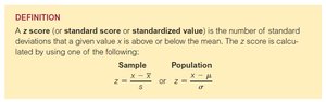
The z-score (also known as standard score or standardized value) is a statistical measure that describes the position of a data value relative to the mean of the dataset, expressed in terms of standard deviations. It is a fundamental concept for comparing values across different distributions and identifying unusual values.

• Definition: The z-score is the number of standard deviations a value x is above or below the mean.

• Formula: For a sample: $z = \frac{x - \bar{x}}{s}$; for a population: $z = \frac{x - \mu}{\sigma}$

• Unitless: z-scores have no units, making them useful for comparison.

• Interpretation: Positive z-scores indicate values above the mean; negative z-scores indicate values below the mean.

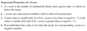
Important Properties of z-Scores

• A z-score quantifies how far a value is from the mean in standard deviation units.

• z-scores are unitless.

• Values with z-scores ≤ -2 or ≥ 2 are considered significantly low or significantly high, respectively.

• If a data value is less than the mean, its z-score is negative.

Identifying Unusual (Significant) Values

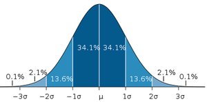
Statisticians often consider values with a probability of 5% or less as unusual. According to the Empirical Rule, values more than two standard deviations from the mean are unusual.

• Unusual values: z-score > 2.00 or z-score < -2.00

• Empirical Rule: 68.2% of values within ±1σ, 95.4% within ±2σ, 99.7% within ±3σ

Percentiles

Percentiles are a popular method for measuring the position of a data value within a dataset. The percentile of a value indicates the percentage of data values below it.

• Definition: The percentile of value x is the percentage of values less than x.

• Formula: $\text{Percentile of value } x = \frac{\text{number of values less than } x}{\text{total number of values}} \times 100$

• Round the result to the nearest whole number.

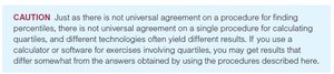
Caution on Percentiles and Quartiles

Note: There is no universal agreement on procedures for calculating percentiles and quartiles. Different calculators or software may yield different results.

Converting a Percentile to a Data Value

To find the data value corresponding to a given percentile, use the locator formula:

• Locator formula: $l = \frac{k}{100} \cdot n$

• k = kth percentile, n = total number of data values

• If the locator is a decimal, round up to the next integer.

• If the locator is a whole number, take the average of that value and the next data value.

Example: Walking Data

Given a list of walking times for 45 students:

To find the 90th percentile (P90):

• Locator: $l = \frac{90}{100} \cdot 45 = 40.5 \rightarrow 41$

• The 41st value is 16.8 min.

Example: Meal Data

For a small dataset of meal prices:

• P50 (Median) = $31, but locator formula gives the 2nd value ($30).

• Locator: $l = \frac{50}{100} \cdot 4 = 2$

• For whole-number locators, average the value and the next data value.

Quartiles and the Five-Number Summary

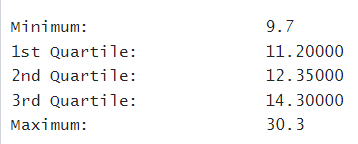
Quartiles divide the data into four equal parts. The Five-Number Summary consists of the minimum, first quartile (Q1), median (Q2), third quartile (Q3), and maximum.

• Q1 = P25 (First Quartile)

• Q2 = P50 (Median)

• Q3 = P75 (Third Quartile)

Statistic	Value
Minimum	9.7
Q1 (25th percentile)	11.2
Median (Q2, 50th percentile)	12.35
Q3 (75th percentile)	14.3
Maximum	30.3

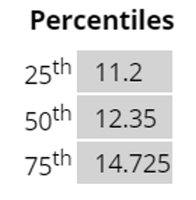
Percentile Table Example

Percentile	Value
25th	11.2
50th	12.35
75th	14.725

Boxplots and Interquartile Range (IQR)

A boxplot (or box-and-whisker plot) visually represents the Five-Number Summary. The Interquartile Range (IQR) is a stable measure of spread, calculated as:

• Formula: $\text{IQR} = Q_3 - Q_1$

• IQR is less affected by extreme values than the range or standard deviation.

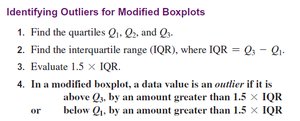
Modified Boxplots and Outliers

Outliers are data values that are far from the rest of the group. Modified boxplots use special symbols to identify outliers and adjust the whiskers to exclude them. The procedure for identifying outliers is:

1. Find quartiles Q1, Q2, Q3.

2. Calculate IQR: $\text{IQR} = Q_3 - Q_1$

3. Evaluate $1.5 \times \text{IQR}$

4. A value is an outlier if it is above $Q_3 + 1.5 \times \text{IQR}$ or below $Q_1 - 1.5 \times \text{IQR}$

Some statistical programs distinguish between mild outliers (outside 1.5 IQRs) and extreme outliers (outside 3 IQRs).

Example: Outlier Identification

For the electricity data, 30.3 is an extreme outlier since it lies outside the upper fence ($Q_3 + 3 \times \text{IQR}$).

Summary Table: Stability of Common Statistics

Stability	Measure of Center	Measure of Variation
Very Unstable	Midrange	Range
Kinda Unstable	Mean	Standard Deviation
Very Stable	Median	IQR

Additional info: These notes expand on the original content by providing definitions, formulas, examples, and tables for clarity and completeness. All images included are directly relevant to the adjacent explanations, reinforcing key concepts in measures of position.