Measures of Variation and Relative Standing in Statistics

Measures of Variation

Concept of Variation

Variation, or dispersion, describes the amount of fluctuation of observations in a data set around their mean. It is a key characteristic of distributions, indicating how spread out the data values are. The difference between each observation and the mean is called a deviation.

Measures of Variation

• Range: The difference between the maximum and minimum values in a data set. It is sensitive to extreme values (outliers).

• Variance: The mean of the squared deviations from the mean. It quantifies the average squared distance of each data value from the mean.

• Standard Deviation: The square root of the variance. It measures the average distance of data values from the mean, in the same units as the original data.

Range

The range is calculated as:

$\text{Range} = \text{Maximum value} - \text{Minimum value}$

While easy to compute, the range is not resistant to outliers and may not accurately reflect the overall variability of the data.

Variance and Standard Deviation

Variance and standard deviation are more robust measures of spread. They are used to determine the spread of data, the number of values within a specified interval, and are foundational in inferential statistics.

Population Variance and Standard Deviation

• Population Variance (σ²): The mean of the squared deviations from the population mean.

• Population Standard Deviation (σ): The square root of the population variance.

Formulas:

$\sigma^2 = \frac{\sum (X - \mu)^2}{N}$

$\sigma = \sqrt{\frac{\sum (X - \mu)^2}{N}}$

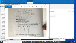
Sample Variance and Standard Deviation

• Sample Variance (s²): An unbiased estimator of the population variance, calculated by dividing by (n-1) instead of n.

• Sample Standard Deviation (s): The square root of the sample variance.

Formulas:

$s^2 = \frac{\sum (X - \overline{X})^2}{n-1}$

$s = \sqrt{\frac{\sum (X - \overline{X})^2}{n-1}}$

Properties of Variance and Standard Deviation

• Always non-negative.

• Smaller values indicate data are closer to the mean; larger values indicate more spread.

• Sensitive to outliers.

• Units: Variance is in squared units; standard deviation is in the same units as the data.

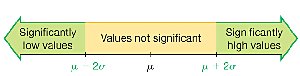
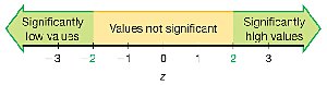
Range Rule of Thumb

The range rule of thumb estimates that most values (about 95%) lie within two standard deviations of the mean:

• Significantly low values: $\mu - 2\sigma$ or lower

• Significantly high values: $\mu + 2\sigma$ or higher

• Values not significant: Between $\mu - 2\sigma$ and $\mu + 2\sigma$

Empirical Rule

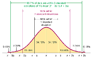
The empirical rule applies to bell-shaped (normal) distributions:

• About 68% of values fall within 1 standard deviation of the mean.

• About 95% within 2 standard deviations.

• About 99.7% within 3 standard deviations.

Chebyshev’s Theorem

Chebyshev’s theorem applies to any data set, regardless of shape. For any number $k > 1$, at least $1 - \frac{1}{k^2}$ of the data values lie within $k$ standard deviations of the mean.

• For $k=2$: At least 75% of values within 2 standard deviations.

• For $k=3$: At least 89% of values within 3 standard deviations.

Coefficient of Variation (CV)

The coefficient of variation expresses the standard deviation as a percentage of the mean, allowing comparison of variability between data sets with different units or means.

Formulas:

• Sample: $CV = \frac{s}{\overline{X}} \times 100\%$

• Population: $CV = \frac{\sigma}{\mu} \times 100\%$

Biased and Unbiased Estimators

• The sample variance $s^2$ is an unbiased estimator of the population variance $\sigma^2$.

• The sample standard deviation $s$ is a biased estimator of the population standard deviation $\sigma$.

Measures of Relative Standing

Z-Scores (Standardized Values)

A z-score indicates how many standard deviations a value $x$ is above or below the mean. It is unitless and allows comparison across different data sets.

• Sample: $z = \frac{x - \overline{X}}{s}$

• Population: $z = \frac{x - \mu}{\sigma}$

Properties:

• z-scores less than -2 or greater than +2 are considered significant (potential outliers).

• z-scores are used to compare relative positions in different distributions.

Percentiles

Percentiles divide a data set into 100 equal parts. The kth percentile is the value below which k percent of the data fall.

Percentile of value x:

$\text{Percentile of } x = \frac{\text{number of values less than } x}{\text{total number of values}} \times 100$

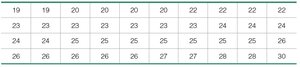
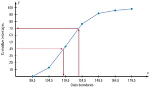
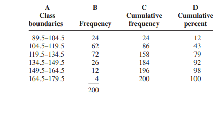
Percentile Graphs and Tables

Percentile graphs (ogives) and tables display cumulative percentages, helping visualize the distribution of data.

Quartiles and Interquartile Range (IQR)

Quartiles divide sorted data into four equal parts:

• Q1: First quartile (25th percentile)

• Q2: Second quartile (median, 50th percentile)

• Q3: Third quartile (75th percentile)

The interquartile range (IQR) is $Q3 - Q1$ and measures the spread of the middle 50% of data.

Outliers and the IQR

Outliers are values that are much higher or lower than the rest of the data. A common rule is:

• Values less than $Q1 - 1.5 \times IQR$ or greater than $Q3 + 1.5 \times IQR$ are considered outliers.

Five-Number Summary and Boxplots

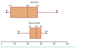
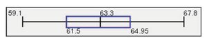
The five-number summary consists of the minimum, Q1, median (Q2), Q3, and maximum. Boxplots (box-and-whisker diagrams) visually display this summary, showing the spread and skewness of the data, and identifying outliers.

Constructing Boxplots

1. Find the five-number summary.

2. Draw a horizontal axis with a scale including the minimum and maximum values.

3. Draw a box from Q1 to Q3, with a line at the median.

4. Draw whiskers from the minimum to Q1 and from Q3 to the maximum.

Notation Summary

• s: Sample standard deviation

• s²: Sample variance

• σ: Population standard deviation

• σ²: Population variance