Normal and Sampling Distributions: Study Guide (Chapters 7 & 8)

Normal Distributions

Properties of the Normal Distribution

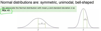
The Normal distribution is a fundamental probability distribution in statistics, used to model data that is symmetric and bell-shaped. It is defined by its mean (μ) and standard deviation (σ), and is widely used due to its mathematical properties and the Central Limit Theorem.

• Symmetry: The curve is symmetric about its mean, μ.

• Single Peak: Mean = median = mode; the highest point is at x = μ.

• Inflection Points: Located at μ – σ and μ + σ.

• Total Area: The area under the curve is 1, representing the total probability.

• Equal Halves: Area to the left and right of μ is each 0.5.

• Asymptotic: The curve approaches, but never touches, the horizontal axis as x → ±∞.

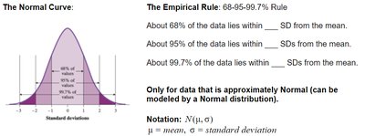
The Empirical Rule (68-95-99.7 Rule)

The Empirical Rule describes the spread of data in a normal distribution:

• About 68% of data lies within 1 standard deviation of the mean.

• About 95% within 2 standard deviations.

• About 99.7% within 3 standard deviations.

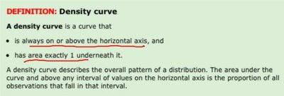
Density Curves

A density curve is a mathematical model that describes the overall pattern of a distribution. It must always be on or above the horizontal axis and have an area of exactly 1 underneath it. The area under the curve over an interval represents the proportion of observations in that interval.

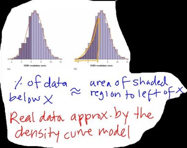
Real Data vs. Model

Real data can be approximated by the density curve model. The proportion of data below a value x is approximately equal to the area under the curve to the left of x.

Notation for Normal Distributions

Normal distributions are denoted as $N(\mu, \sigma)$, where μ is the mean and σ is the standard deviation.

Standardization and the Standard Normal Distribution

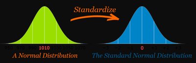
Why Standardize?

Standardizing allows us to compare values from different normal distributions and use a single table (the z-table) for probability calculations. This process converts any normal distribution to the standard normal distribution, which has a mean of 0 and a standard deviation of 1.

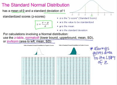
Calculating Z-scores

The z-score for a value x is calculated as:

$z = \frac{x - \mu}{\sigma}$

This score tells us how many standard deviations x is from the mean.

The Standard Normal Distribution

The standard normal distribution is denoted as $N(0, 1)$. Probabilities are found using the z-table, which gives the area to the left of a given z-score.

Sampling Distributions

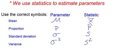
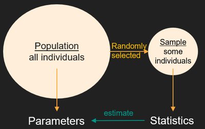
Parameters vs. Statistics

A parameter is a value that describes a population (usually unknown), while a statistic is a value calculated from a sample (random variable). We use statistics to estimate parameters.

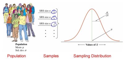
Sampling Distribution of the Sample Mean

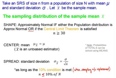
The sampling distribution of the sample mean ($\overline{x}$) is the distribution of sample means from all possible samples of a given size from the population.

• Shape: Approximately normal if the population is normal or if the sample size is large (Central Limit Theorem: $n \geq 30$).

• Center: Mean of the sampling distribution is $\mu_{\overline{x}} = \mu$ (unbiased estimator).

• Spread: Standard deviation is $\sigma_{\overline{x}} = \frac{\sigma}{\sqrt{n}}$, provided the sample size is less than 10% of the population (when sampling without replacement).

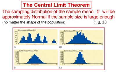
The Central Limit Theorem (CLT)

The CLT states that the sampling distribution of the sample mean will be approximately normal if the sample size is large enough ($n \geq 30$), regardless of the population's shape.

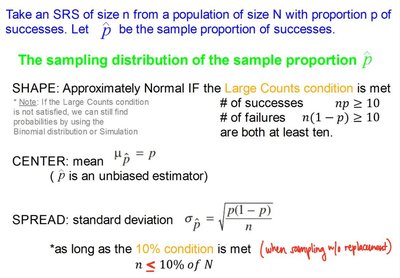
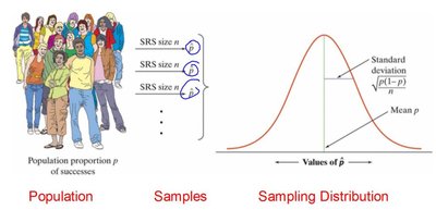
Sampling Distribution of the Sample Proportion

The sampling distribution of the sample proportion ($\hat{p}$) describes the distribution of sample proportions from all possible samples of a given size.

Shape: Approximately normal if the Large Counts condition is met: $np \geq 10$ and $n(1-p) \geq 10$.

• Center: Mean is $\mu_{\hat{p}} = p$ (unbiased estimator).

• Spread: Standard deviation is $\sigma_{\hat{p}} = \sqrt{\frac{p(1-p)}{n}}$, provided $n \leq 0.1N$ (10% condition).

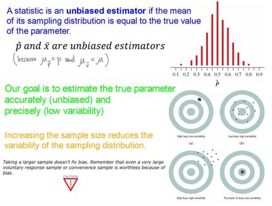
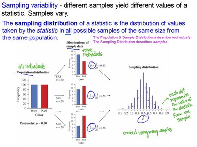
Sampling Variability and Unbiased Estimators

Different samples yield different statistics due to sampling variability. A statistic is an unbiased estimator if its mean equals the true parameter value. Increasing sample size reduces the variability of the sampling distribution.

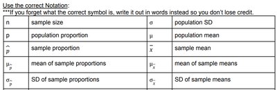
Notation Reference Table

Correct notation is essential in statistics. The following table summarizes key symbols:

Symbol	Meaning
n	Sample size
p	Population proportion
\hat{p}	Sample proportion
\mu	Population mean
\overline{x}	Sample mean
\mu_{\hat{p}}	Mean of sample proportions
\mu_{\overline{x}}	Mean of sample means
\sigma	Population standard deviation
S	Sample standard deviation
\sigma_{\hat{p}}	SD of sample proportions
\sigma_{\overline{x}}	SD of sample means

Additional info: For exam preparation, practice problems are essential. Redo exercises from your textbook, online platforms, and review Kahoot or Pearson assignments for mastery.