Normal and Uniform Probability Distributions: Concepts, Calculations, and Applications

Normal Probability Distributions

Definition and Properties of the Normal Distribution

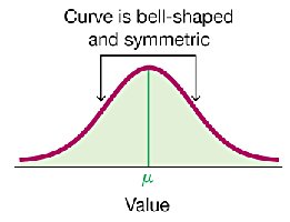
The normal distribution is a continuous probability distribution characterized by a symmetric, bell-shaped curve. It is defined by two parameters: the mean (\( \mu \)) and the standard deviation (\( \sigma \)). The normal distribution is fundamental in statistics due to its natural occurrence in many real-world phenomena and its mathematical properties.

• Bell-shaped and symmetric: The curve is highest at the mean and decreases symmetrically on both sides.

• Mean (\( \mu \)): The center of the distribution.

• Standard deviation (\( \sigma \)): Measures the spread or dispersion of the distribution.

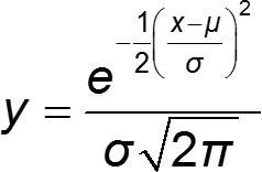
The probability density function (PDF) for the normal distribution is:

$y = \frac{e^{-\frac{1}{2}\left(\frac{x-\mu}{\sigma}\right)^2}}{\sigma \sqrt{2\pi}}$

The Standard Normal Distribution

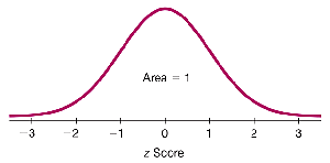
The standard normal distribution is a special case of the normal distribution with a mean of 0 and a standard deviation of 1. It is denoted by the variable z and is used to standardize values from any normal distribution for comparison.

• Mean (\( \mu \)) = 0

• Standard deviation (\( \sigma \)) = 1

• Total area under the curve = 1

Density Curves and Area-Probability Correspondence

The graph of any continuous probability distribution is called a density curve. The total area under a density curve is exactly 1, establishing a direct correspondence between area and probability. For the normal distribution, probabilities are found by calculating the area under the curve for a given interval.

Uniform Probability Distributions

Definition and Properties of the Uniform Distribution

A uniform distribution is a continuous probability distribution where all outcomes in a certain interval are equally likely. The graph of a uniform distribution is a rectangle, and the area under the curve is always 1.

• All values are equally likely within the interval.

• Area under the curve = 1

• Probability = Area = height × width

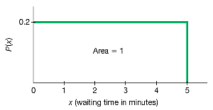
In general, the height of the rectangle is \( \frac{1}{\text{range}} \).

Example: Waiting Times for Airport Security

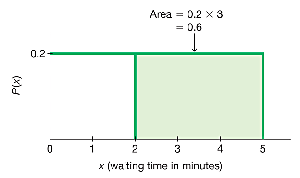
Suppose waiting times at an airport security checkpoint are uniformly distributed between 0 and 5 minutes. The probability that a randomly selected passenger waits at least 2 minutes is calculated by finding the area of the rectangle from 2 to 5 minutes.

• Height = 0.2 (since \( \frac{1}{5-0} = 0.2 \))

• Width = 3 (from 2 to 5 minutes)

• Probability = 0.2 × 3 = 0.6

Finding Probabilities and Areas Under the Normal Curve

z Scores and Their Interpretation

A z score represents the number of standard deviations a value is from the mean. It is calculated as:

$z = \frac{x - \mu}{\sigma}$

z scores allow comparison of values from different normal distributions by standardizing them.

Using Technology and Tables

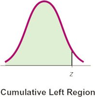
Probabilities (areas) under the normal curve can be found using statistical tables (such as Table A-2) or technology (Excel, calculators). Table A-2 provides cumulative areas from the left up to a given z score.

Example: Bone Density Test

Suppose bone density z scores are normally distributed with mean 0 and standard deviation 1. To find the probability that a randomly selected person has a z score less than 1.27:

• Use Excel: NORM.S.DIST(1.27, TRUE)

• Result: 0.8980 (rounded)

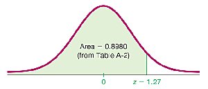
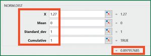
This means 89.80% of people have bone density below 1.27.

Finding Areas to the Right or Between Values

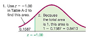
To find the probability above a certain z value, subtract the cumulative area from 1. For example, the probability above z = -1.00 is 1 - 0.1587 = 0.8413.

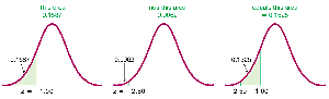
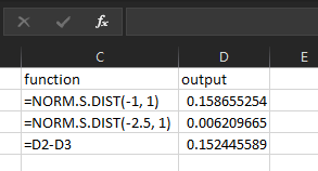
To find the probability between two z values, subtract the cumulative area for the lower z from the cumulative area for the higher z.

Notation for Probabilities

• P(a < z < b): Probability z is between a and b

• P(z > a): Probability z is greater than a

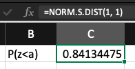
• P(z < a): Probability z is less than a

Finding z Scores from Known Areas

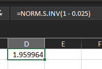
To find a z score corresponding to a given cumulative area (probability), use the inverse normal function in technology (e.g., NORM.S.INV in Excel) or locate the closest probability in the body of Table A-2 and read the corresponding z score.

Critical Values in the Standard Normal Distribution

Definition and Notation

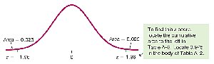
A critical value is a z score that separates significantly low or high values from the rest of the distribution. The notation z\( \alpha \) denotes the z score with an area of \( \alpha \) to its right.

• To find z\( \alpha \), use the cumulative area to the left: 1 - \( \alpha \).

• For example, z0.025 is the z score with 0.025 area to its right (or 0.975 to its left), which is approximately 1.96.

Summary Table: Key Properties of Normal and Uniform Distributions

Distribution	Shape	Parameters	Probability Calculation
Normal	Bell-shaped, symmetric	Mean (\( \mu \)), Std. Dev. (\( \sigma \))	Area under curve (integral or table/technology)
Uniform	Rectangular	Lower and upper bounds (a, b)	Area = height × width; height = \( \frac{1}{b-a} \)