Normal Distribution and Sampling Distribution of Means

Normal Distribution and Sampling Distribution of Means

Probability Density Function

A probability density function (PDF) is a function used to compute probabilities for continuous random variables. It must satisfy two properties:

• The graph of the function must lie on or above the horizontal axis.

• The total area under the graph must be 1.

This ensures that the PDF represents a valid probability distribution for continuous data.

Normal Distribution

The normal distribution is a continuous probability distribution characterized by its bell-shaped, symmetric curve. It is also known as the Gaussian distribution, named after Carl Gauss, and is widely used to model natural phenomena.

• The normal distribution is defined for all real numbers: $-\infty < x < +\infty$.

• It is described by two parameters: the mean ($\mu$) and the standard deviation ($\sigma$).

• The notation for a normal distribution is $N(\mu, \sigma)$ or $N(\mu, \sigma^2)$.

• Example: $N(20, 3)$ or $N(20, 3^2)$.

Features of the Normal Curve

The normal curve has several important features:

• It is bell-shaped and symmetric about the mean ($\mu$).

• The mean, median, and mode are all equal and located at the center of the distribution.

• The curve approaches, but never touches, the horizontal axis.

• As the standard deviation ($\sigma$) increases, the curve becomes wider and flatter; as $\sigma$ decreases, the curve becomes narrower and more peaked.

Normal Distribution Function

The probability density function for the normal distribution is given by:

$f(x; \mu, \sigma) = \frac{1}{\sigma \sqrt{2\pi}} e^{-\frac{(x-\mu)^2}{2\sigma^2}}$

• $\mu$ is the population mean.

• $\sigma$ is the population standard deviation.

This function describes the likelihood of a random variable taking a particular value in a normal distribution.

Normal Probability and Area Under the Curve

The area under the normal curve within a given interval represents the probability that a measurement will fall within that interval. The total area under the curve is 1, meaning:

• 50% of the data lies to the left of the mean ($\mu$).

• 50% of the data lies to the right of the mean ($\mu$).

Ways to Identify Normality in Data

There are several methods to determine if a dataset is approximately normal:

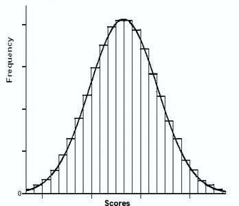
• Histogram: A normal distribution's histogram should be roughly bell-shaped.

• Outliers: A normal distribution should have no more than one outlier.

• Quantile-Quantile (QQ) Plot: If the data points lie close to a straight line, the data is approximately normal.

Empirical Rule (68-95-99.7 Rule)

The empirical rule describes how data is distributed in a normal distribution:

• About 68% of the data falls within one standard deviation of the mean ($\mu \pm \sigma$).

• About 95% of the data falls within two standard deviations of the mean ($\mu \pm 2\sigma$).

• About 99.7% of the data falls within three standard deviations of the mean ($\mu \pm 3\sigma$).

This rule is useful for quickly estimating probabilities and identifying outliers in normally distributed data.