Normal Probability Distribution: Concepts, Calculations, and Applications

Normal Probability Distribution

Continuous Random Variables

Continuous random variables are variables that can take any real value within a given interval. Unlike discrete random variables, their possible values cannot be listed exhaustively because there are infinitely many possibilities within any range.

• Definition: A continuous random variable is one that can assume any value in an interval on the real number line.

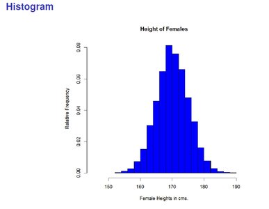
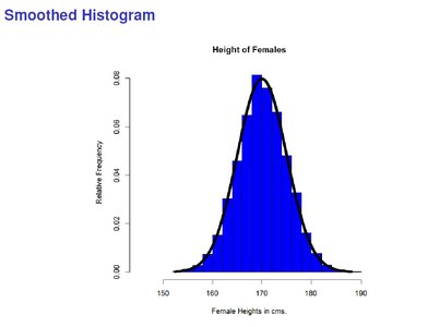
• Examples: Height, weight, age, time, temperature, pressure, and pH are all examples of continuous random variables.

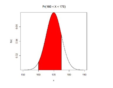
• Probability Statements: For a specific value, the probability is zero: $P(X = x) = 0$. Instead, probabilities are calculated over intervals, such as $P(X \geq a)$, $P(X \leq b)$, or $P(a \leq X \leq b)$.

Density Curves

A density curve is a graphical representation of the probability distribution of a continuous random variable. The area under the curve over an interval represents the probability that the variable falls within that interval.

• Properties: The total area under a density curve is always 1.

• Interpretation: The curve never drops below the horizontal axis, and the area under the curve between two values gives the probability of the variable falling within that range.

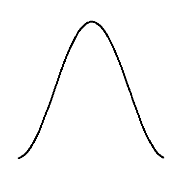
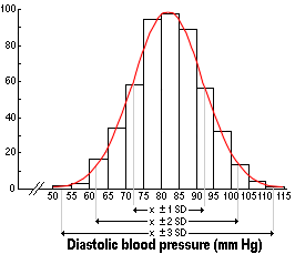
The Normal Probability Distribution

The normal distribution is a continuous probability distribution that is symmetric and bell-shaped. It is defined by its mean ($\mu$) and standard deviation ($\sigma$).

• Characteristics:

  • The mean, median, and mode are all equal and located at the center of the distribution.

  • The curve is symmetric about the mean.

  • The standard deviation determines the spread (width) of the curve.

  • The total area under the curve is 1.

• Equation: The probability density function (PDF) for the normal distribution is: $$ f(x) = \frac{1}{\sigma \sqrt{2\pi}} e^{-\frac{1}{2} \left( \frac{x-\mu}{\sigma} \right)^2}$$

Effect of Standard Deviation

• A smaller $\sigma$ results in a narrower, taller curve.

• A larger $\sigma$ results in a wider, flatter curve.

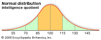
Example: IQ Scores

• IQ scores are normally distributed with $\mu = 100$ and $\sigma = 15$.

• To find the percentage of people with IQ above 130, calculate $P(X > 130)$ using the normal distribution.

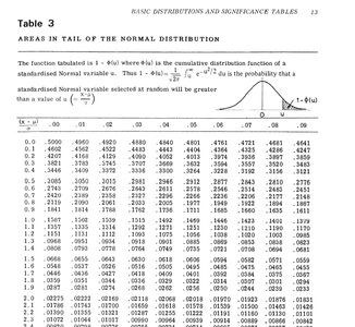
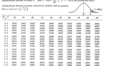
The Standard Normal Distribution (Z-Distribution)

The standard normal distribution is a special case of the normal distribution with a mean of 0 and a standard deviation of 1. Probabilities for any normal distribution can be found by converting values to the standard normal distribution using the z-score formula.

• Z-Score Formula: $$ Z = \frac{X - \mu}{\sigma}$$

• Interpretation: The z-score represents the number of standard deviations a value is from the mean.

• Z-Tables: Standard normal tables (Z-tables) provide the probability that a standard normal variable is less than or greater than a given value.

Empirical Rule (68-95-99.7 Rule)

• Approximately 68% of values fall within 1 standard deviation of the mean.

• Approximately 95% of values fall within 1.96 standard deviations of the mean.

• Approximately 99.7% of values fall within 3 standard deviations of the mean.

Transforming to the Standard Normal Distribution

• Any value from a normal distribution can be converted to a z-score using the formula above.

• Once converted, use the Z-table to find probabilities.

Worked Examples

• IQ Example: What percentage of people have an IQ score above 125?

• Foal Birth Weights: Mean = 54kg, $\sigma$ = 6.3kg

  • (i) Percentage above 65kg

  • (ii) Percentage below 50kg

  • (iii) Percentage between 52kg and 60kg

  • (iv) The value below which the smallest 10% of foals fall

• Junior Doctors' Weekly Hours: Mean = 45 hours, $\sigma$ = 5 hours

  • (i) Proportion working more than 50 hours

  • (ii) Proportion working less than 36 hours

  • (iii) Number of hours only 5% exceed

  • (iv) Proportion working between 40 and 50 hours

Applications of the Normal Distribution

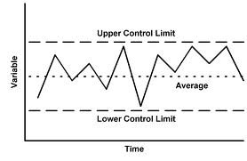
1. Control Charts

Control charts are used in quality control to monitor whether a process is in a state of statistical control. For a normally distributed process, over 99% of observations fall within 3 standard deviations of the mean.

• Upper Control Limit (UCL): $\mu + 3\sigma$

• Lower Control Limit (LCL): $\mu - 3\sigma$

• Observations outside these limits are considered unusual and may indicate a problem with the process.

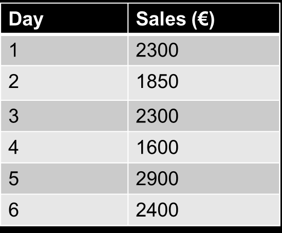
Example: Restaurant Daily Sales

• Mean daily sales: €2100, $\sigma$ = €250

• Data for 6 days is given. Calculate UCL and LCL, and identify unusual observations.

Day	Sales (€)
1	2300
2	1850
3	2300
4	1600
5	2900
6	2400

2. Using Z-values to Identify Unusual Cases

Z-values can be used to compare individual observations to the population and identify outliers or unusual cases.

• Example: Diastolic blood pressure in adult males is normally distributed with mean 83 mmHg and $\sigma$ = 10 mmHg. A patient with a blood pressure of 125 mmHg can be compared to the population using the z-score.

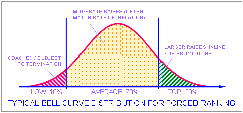
3. Employee Appraisals

Normal distribution can be used for forced ranking in large groups, where employees are ranked based on their performance relative to the group. This method is less effective for small teams.

Summary

• The normal distribution is defined by its mean and standard deviation.

• The Z-table provides probabilities for the standard normal distribution.

• Any value from a normal distribution can be transformed to a z-value using $Z = \frac{X - \mu}{\sigma}$.