CH. 6 Normal Probability Distributions and Sampling Distributions: Study Guide

Normal Probability Distributions

Density Curves and Continuous Probability Distributions

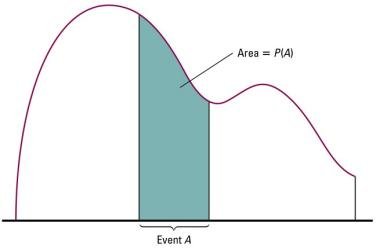
In statistics, a density curve is a smooth curve that represents the distribution of a continuous variable. The area under the curve for a given interval represents the probability of the variable falling within that interval. The function describing the density curve is called the probability density function (p.d.f.).

• Continuous Probability Distribution: Satisfies three conditions:

  1. The random variable is continuous.

  2. The probability density function f(x) ≥ 0 for all x.

  3. The total area under the p.d.f. curve is 1.

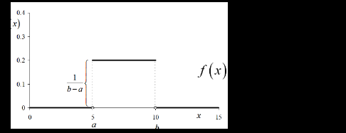
Uniform Distribution

A uniform distribution is a continuous probability distribution where all outcomes are equally likely within a certain interval [a, b]. The graph of a uniform distribution is rectangular.

• Probability Density Function: $f(x) = \begin{cases} \frac{1}{b-a} & \text{if } a \leq x \leq b \\ 0 & \text{otherwise} \end{cases}$

• Area Calculation: Area = height × width

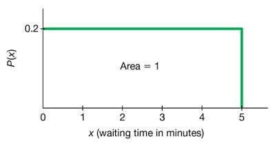
Example: Waiting Time at Subway

• Waiting time is uniformly distributed between 0 and 5 minutes.

• Height of the distribution: $\text{Height} = \frac{1}{5} = 0.2$

• Probability of waiting more than 2 minutes: $P(X > 2) = 0.2 \times (5-2) = 0.6$

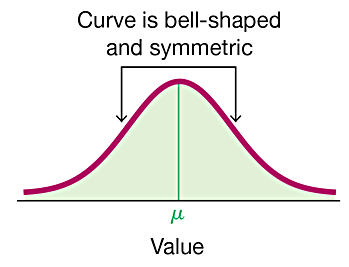
Normal Distribution

A normal distribution is a continuous probability distribution characterized by its bell-shaped, symmetric curve. It is defined by its mean (μ) and standard deviation (σ).

• Symmetric about the mean μ.

• The spread depends on σ; larger σ means a flatter, more spread-out curve.

• Probability density function: $y = \frac{e^{-\frac{1}{2} \left( \frac{x-\mu}{\sigma} \right)^2}}{\sigma \sqrt{2\pi}}$

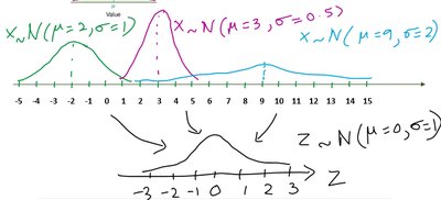
Standard Normal Distribution

The standard normal distribution is a normal distribution with mean 0 and standard deviation 1. Values from any normal distribution can be standardized using the z-score formula.

• Standard normal curve is used to find probabilities and percentiles.

• Z-score formula: $z = \frac{x - \mu}{\sigma}$

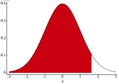
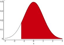
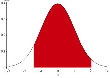
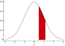
Finding Probabilities Using the Normal Distribution

Probabilities are found by calculating the area under the normal curve for a given range of values.

• Use statistical software (e.g., StatCrunch) or tables to find probabilities for given z or x values.

• For probability between two values: $P(a \leq x \leq b)$, calculate the area between a and b.

Example: Toyota Car Battery Lifetime

• Mean = 45 months, σ = 8 months

• Probability battery fails within 36 months: $P(X \leq 36) = 0.13$

• Probability battery lasts between 36 and 50 months: $P(36 \leq X \leq 50) = 0.60$

• Probability battery lasts 55 months or longer: $P(X \geq 55) = 0.11$

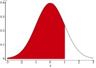
Visualizing Probabilities on the Normal Curve

Shaded regions on the normal curve represent the probability for a given range.

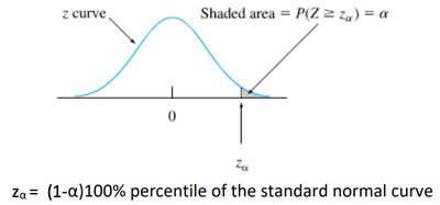
Percentiles and Critical Values

Percentiles and critical values are important for hypothesis testing and confidence intervals.

• Given a probability (area), find the corresponding z-score or x value.

• 95th percentile (P95): $z = 1.645$

• Critical value $z_\alpha$: The z-score for which the area to the right is α.

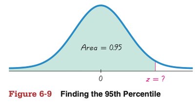
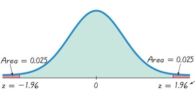
Example: Bone Density Score

• Find the score corresponding to the 95th percentile: $z = 1.645$

• Find scores separating the bottom and top 2.5%: $z = -1.96$ and $z = 1.96$

Sampling Distributions and Estimators

Sampling Distribution of the Sample Mean

The sampling distribution of a statistic is the probability distribution of that statistic based on all possible samples from the population.

• The mean of the sample means equals the population mean: $\mu_{\bar{x}} = \mu$

• The standard deviation of the sample means: $\sigma_{\bar{x}} = \frac{\sigma}{\sqrt{n}}$

Example: Heights of Students

Sample	Heights	Sample Mean (𝑥̅)
A,B	76,78	77.0
A,C	76,79	77.5
A,D	76,81	78.5
A,E	76,86	81.0
B,C	78,79	78.5
B,D	78,81	79.5
B,E	78,86	82.0
C,D	79,81	80.0
C,E	79,86	82.5
D,E	81,86	83.5

Sampling Distribution of Sample Proportion

The sampling distribution of sample proportion describes the distribution of sample proportions from all possible samples.

• Sample proportion: $\hat{p} = \frac{x}{n}$

• Population proportion: $p = \frac{x}{N}$

• Mean: $p$

• Standard deviation: $\sigma_{\hat{p}} = \sqrt{\frac{p(1-p)}{n}}$

• Shape is normal if $np \geq 5$ and $n(1-p) \geq 5$

Central Limit Theorem

Statement and Applications

The Central Limit Theorem (CLT) states that if the sample size is large enough (n ≥ 30), the sampling distribution of the sample mean is approximately normal, regardless of the population's distribution.

• If population is normal: $\bar{x} \sim N(\mu, \frac{\sigma^2}{n})$

• If n ≥ 30: $\bar{x} \sim N(\mu, \frac{\sigma^2}{n})$

• For individual values: $z = \frac{x - \mu}{\sigma}$

• For sample means: $z = \frac{\bar{x} - \mu}{\sigma / \sqrt{n}}$

Example: Water Taxi Capacity

• Mean weight of men: 182.9 lb, σ = 40.8 lb

• Probability individual man weighs > 140 lb: $P(X > 140) = 0.853$

• Probability average weight of 25 men > 140 lb: $P(\bar{X} > 140) = 1$

• Conclusion: Capacity is not safe; probability of overloading is 1.

Example: SAT Scores

• Mean = 1511, σ = 312

• Probability individual score > 1600: $P(X > 1600) = 0.388$

• Probability average score of 36 students > 1600: $P(\bar{X} > 1600) = 0.043$

• 98th percentile for average score of 45 students: $a = 1606.52$

Summary Table: Key Formulas

Concept	Formula
Z-score (individual)	$z = \frac{x - \mu}{\sigma}$
Z-score (sample mean)	$z = \frac{\bar{x} - \mu}{\sigma / \sqrt{n}}$
Sample mean std. dev.	$\sigma_{\bar{x}} = \frac{\sigma}{\sqrt{n}}$
Sample proportion std. dev.	$\sigma_{\hat{p}} = \sqrt{\frac{p(1-p)}{n}}$
Uniform distribution p.d.f.	$f(x) = \frac{1}{b-a}$ for $a \leq x \leq b$
Normal distribution p.d.f.	$y = \frac{e^{-\frac{1}{2} \left( \frac{x-\mu}{\sigma} \right)^2}}{\sigma \sqrt{2\pi}}$