Normal Probability Distributions and Sampling Distributions: Study Notes

Ch. 5 - Normal Probability Distributions

Standard Normal Distribution

The standard normal distribution is a normal distribution with a mean of 0 and a standard deviation of 1. Probabilities for this distribution are found using the z-table, which gives the area (probability) to the left of a given z-score.

• Z-score (z): The number of standard deviations a value is from the mean.

• Probability and Area: For continuous random variables, probability is the area under the density curve.

• Using the Z-table: The table always shows cumulative areas to the left of the z-score.

Example: To find P(Z < -0.64), look up -0.64 in the z-table to get the area to the left. To find P(Z > 2.27), subtract the area to the left of 2.27 from 1.

Finding Areas Under the Standard Normal Curve

• Area to the Right: P(Z > z) = 1 - P(Z < z)

• Area Between Two Z-scores: Subtract the area to the left of the smaller z-score from the area to the left of the larger z-score.

Example: P(-0.64 < Z < 2.27) = P(Z < 2.27) - P(Z < -0.64)

Finding Z-Scores from Probabilities

To find a z-score given a probability (area), use the z-table in reverse. If the area is to the right, subtract from 1 to get the area to the left, then look up the corresponding z-score.

• Given Area to Left: Find the z-score whose cumulative area matches the given probability.

• Given Area to Right: Subtract the probability from 1, then find the corresponding z-score.

Using the Z-Table

The z-table provides cumulative probabilities for z-scores. For example, the area to the left of z = 0 is 0.5000. The table is symmetric about z = 0.

Standard Normal Distribution with Graphing Calculator

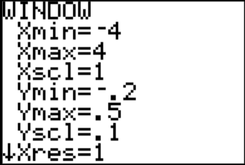
Graphing calculators (e.g., TI-84) can quickly find probabilities and z-scores using functions like normalcdf (for probabilities) and invNorm (for z-scores from probabilities).

• normalcdf(lower, upper, μ, σ): Finds the probability between two bounds.

• invNorm(area, μ, σ): Finds the z-score for a given cumulative area.

Intro to Continuous Random Variables

Discrete vs. Continuous Probability Distributions

Discrete random variables take on countable values (e.g., rolling a die). Continuous random variables can take any value in an interval (e.g., time, distance).

• Discrete Probability: Probability is the sum of probabilities for individual outcomes.

• Continuous Probability Density: Probability is the area under the probability density function (PDF) over an interval.

Uniform Distribution: A continuous distribution where all intervals of the same length are equally likely. The PDF is constant.

Non-Standard Normal Distributions

Finding Z-Scores for Non-Standard Normal Variables

For a normal distribution with mean μ and standard deviation σ, convert any value x to a z-score using:

$z = \frac{x - \mu}{\sigma}$

• Use the standard normal table or calculator to find probabilities for non-standard normal variables by first converting to z-scores.

Finding Values from Probabilities

To find the value x corresponding to a given probability, first find the z-score from the table, then solve for x:

$x = z \cdot \sigma + \mu$

Sampling Distribution for Sample Mean & Central Limit Theorem

Sampling Distribution of the Mean

The sampling distribution of the sample mean is the probability distribution of all possible sample means for samples of a given size n from a population.

• Central Limit Theorem (CLT): For any population, as the sample size n increases, the sampling distribution of the sample mean approaches a normal distribution, regardless of the population's shape.

• For n ≥ 30, the sampling distribution is approximately normal.

Calculating Z-Scores for Sample Means

For a sample mean $\bar{x}$, the z-score is:

$z = \frac{\bar{x} - \mu_{\bar{x}}}{\sigma_{\bar{x}}}$

where $\mu_{\bar{x}}$ is the mean of the sampling distribution and $\sigma_{\bar{x}}$ is the standard error ($\sigma / \sqrt{n}$).

Sampling Distribution of Sample Proportion

Normal Approximation to the Binomial

For a binomial variable with n trials and probability p, if both np ≥ 5 and n(1-p) ≥ 5, the distribution of the sample proportion $\hat{p}$ is approximately normal.

• Continuity Correction: When approximating a discrete binomial with a continuous normal, add or subtract 0.5 as appropriate.

• Sample Proportion: $\hat{p} = \frac{x}{n}$, where x is the number of successes in n trials.

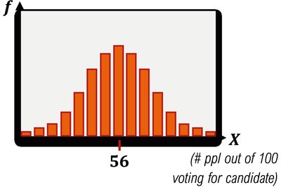
Sampling Distribution of Sample Proportion

The mean of the sampling distribution of $\hat{p}$ is p, and the standard deviation is $\sqrt{\frac{p(1-p)}{n}}$.

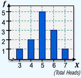
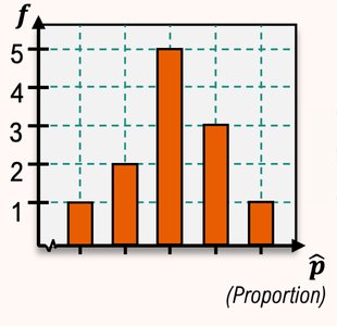
Example: If 80% of people prefer Pepsi, in a sample of 100, the probability that at least 60 prefer Pepsi can be approximated using the normal distribution for $\hat{p}$.

Additional info: The notes above include all main concepts, formulas, and relevant images for Ch. 5 - Normal Probability Distributions, including standard and non-standard normal distributions, the Central Limit Theorem, and the normal approximation to the binomial. All images included directly reinforce the adjacent explanations.