Normal Probability Distributions and the Central Limit Theorem

Chapter 6: Normal Probability Distributions

6.1 The Standard Normal Distribution

The study of probability distributions is fundamental in statistics, especially for continuous random variables. The normal distribution is one of the most important probability distributions due to its prevalence in natural and social phenomena.

Density Curves and Probability Density Functions (p.d.f.)

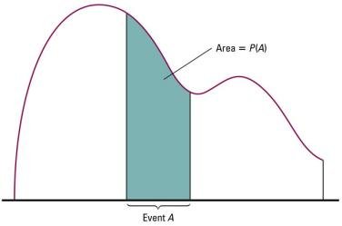
• Density curve: A smooth curve that represents the distribution of a continuous variable. The area under the curve for a given interval represents the probability of the variable falling within that interval.

• Probability density function (p.d.f.): The function that defines the density curve. For a continuous random variable, the probability that the variable falls within a certain interval is the area under the p.d.f. over that interval.

Continuous Probability Distribution

• The random variable is continuous.

• The p.d.f. satisfies $f(x) \geq 0$ for all $x$.

• The total area under the p.d.f. curve is 1: $\int_{-\infty}^{\infty} f(x) dx = 1$.

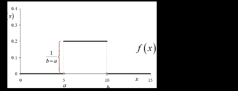
Uniform Distribution

A uniform distribution is a continuous probability distribution where all outcomes are equally likely within a certain interval $[a, b]$. The graph is a rectangle.

• p.d.f.: $f(x) = \begin{cases} \frac{1}{b-a} & a \leq x \leq b \\ 0 & \text{otherwise} \end{cases}$

• Area under the curve: $\text{Area} = \text{height} \times \text{width}$

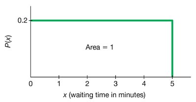
Example: Uniform Distribution

Suppose the waiting time at a restaurant is uniformly distributed between 0 and 5 minutes.

• Height of the distribution: $\text{Area} = \text{Height} \times (5-0) = 1 \implies \text{Height} = \frac{1}{5} = 0.2$

• Probability of waiting more than 2 minutes: $P(X > 2) = 0.2 \times (5-2) = 0.6$

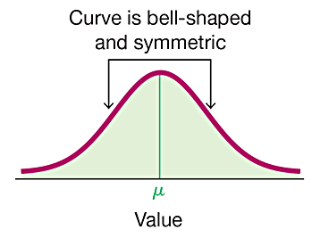
Normal Distribution

A variable is normally distributed if its distribution forms a bell-shaped curve, determined by its mean ($\mu$) and standard deviation ($\sigma$).

• Symmetric about the mean $\mu$.

• The spread depends on $\sigma$; larger $\sigma$ means a flatter, more spread-out curve.

• Probability density function: $f(x) = \frac{1}{\sigma \sqrt{2\pi}} e^{-\frac{1}{2} \left(\frac{x-\mu}{\sigma}\right)^2}$

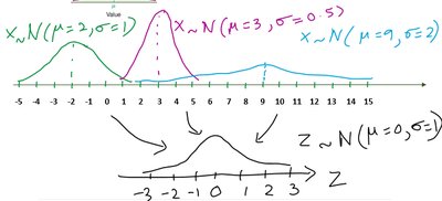
Standard Normal Distribution

The standard normal distribution is a special case of the normal distribution with mean 0 and standard deviation 1. Any normal variable can be standardized using the z-score:

• $z = \frac{x - \mu}{\sigma}$

• The standard normal curve is used to find probabilities and percentiles for any normal distribution.

6.2 Real Applications of Normal Distributions

Probabilities for normal distributions are found by calculating the area under the curve for a given interval. This can be done using statistical software or standard normal tables.

Finding Probabilities

• Given $x$, convert to $z$ using $z = \frac{x - \mu}{\sigma}$.

• Use the standard normal table or software to find $P(X \leq x)$ or $P(Z \leq z)$.

Example: Car Battery Lifetime

• Mean = 45 months, SD = 8 months.

• Probability battery fails within 36 months: $P(X \leq 36) = 0.13$

• Probability battery lasts between 36 and 50 months: $P(36 \leq X \leq 50) = 0.60$

• Probability battery lasts 55 months or longer: $P(X \geq 55) = 0.11$

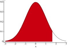
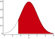
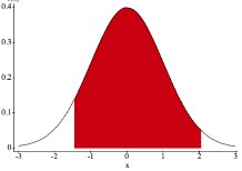
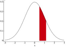
Visualizing Probabilities on the Normal Curve

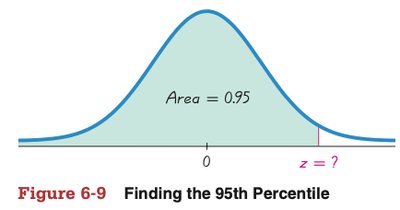
Finding z or x Value Given a Probability (Area)

• Given a probability (area), find the corresponding z-score or x value using the inverse normal function.

• Example: For the 95th percentile, $z = 1.645$.

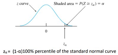
Critical Values ($z_\alpha$)

• A critical value is a z-score that separates the region of significance in hypothesis testing.

• $z_\alpha$ is the z-score such that the area to the right is $\alpha$.

6.3 Sampling Distributions and Estimators

Sampling distributions describe the probability distribution of a statistic (such as the sample mean or proportion) based on all possible samples from a population.

Sampling Distribution of the Sample Mean

• The mean of the sample means ($\mu_{\bar{x}}$) equals the population mean ($\mu$).

• The standard deviation of the sample means ($\sigma_{\bar{x}}$) is $\frac{\sigma}{\sqrt{n}}$.

Sampling Distribution of the Sample Proportion

• Sample proportion: $\hat{p} = \frac{x}{n}$

• Population proportion: $p = \frac{x}{N}$

• Mean of sampling distribution: $p$

• Standard deviation: $\sigma_{\hat{p}} = \sqrt{\frac{p(1-p)}{n}}$

• Shape is approximately normal if $np \geq 5$ and $n(1-p) \geq 5$

6.4 Central Limit Theorem (CLT)

The Central Limit Theorem states that, for a sufficiently large sample size ($n \geq 30$), the sampling distribution of the sample mean is approximately normal, regardless of the population's distribution.

• If the population is normal: $\bar{x} \sim N(\mu, \frac{\sigma^2}{n})$

• If the sample size is large: $\bar{x} \sim N(\mu, \frac{\sigma^2}{n})$

• For individual values: $z = \frac{x - \mu}{\sigma}$

• For sample means: $z = \frac{\bar{x} - \mu}{\sigma/\sqrt{n}}$

Example: Water Taxi Safety

• Mean weight of men: 182.9 lb, SD: 40.8 lb, $n = 25$

• Probability a single man weighs more than 140 lb: $P(X > 140) = 0.853$

• Probability the average weight of 25 men exceeds 140 lb: $P(\bar{X} > 140) = 1$

• Conclusion: The boat's capacity is not safe.

Example: SAT Scores

• Mean = 1511, SD = 312

• Probability a student scores above 1600: $P(X > 1600) = 0.388$

• Probability the average of 36 students is above 1600: $P(\bar{X} > 1600) = 0.043$

• 98th percentile for a class of 45: $a = 1606.52$