Normal Probability Distributions and the Central Limit Theorem: Study Notes

Normal Probability Distributions

Introduction to Normal Distributions

The normal distribution is a fundamental concept in statistics, describing a continuous probability distribution for a random variable, x. Its graph, known as the normal curve, is bell-shaped and symmetric about the mean (μ). The total area under the curve is always 1, representing the entire probability space.

• Mean (μ) and Standard Deviation (σ): A normal distribution can have any mean and any positive standard deviation.

• Shape: Large standard deviation produces a 'fat' curve, while a small standard deviation produces a 'skinny' curve.

The Standard Normal Distribution

The standard normal distribution is a special case of the normal distribution with a mean of 0 and a standard deviation of 1. The variable z represents the number of standard deviations a value is from the mean.

• Properties: The area under the curve to the left of z = 0 is 0.5. Areas to the left of extreme z-scores (e.g., z = -3.49 or z = 3.49) are close to 0 or 1, respectively.

Finding Area Under a Normal Curve

To find the cumulative area (probability) to the left, right, or between z-scores, use the Standard Normal Table or a calculator. The area represents the probability that a randomly selected value falls within a specified range.

• To the left of z: Find the area directly from the table.

• To the right of z: Subtract the area to the left from 1.

• Between two z-scores: Subtract the area to the left of the lower z-score from the area to the left of the higher z-score.

Example: Using The Standard Normal Table

Find the cumulative area that corresponds to a z-score of 1.15. The area to the left of z = 1.15 is 0.8749.

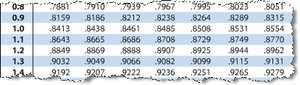
Example: Finding Area Under the Standard Normal Curve

• Area to the left of z = -0.24 is 0.4052.

• Area to the left of z = -0.99 is 0.1611.

• Area to the right of z = 1.06 is 1 - 0.8554 = 0.1446.

• Area between z = -1.50 and z = 1.25 is 0.8944 - 0.0668 = 0.8276.

Normal Distributions: Finding Probabilities

Probability and Normal Distributions

If a random variable x is normally distributed, the probability that x falls within an interval is equal to the area under the normal curve for that interval. To solve these problems, convert x to a z-score using:

• $z = \frac{x - \mu}{\sigma}$

Then use the standard normal table to find the corresponding area.

Example: Cellular Phone Usage

• Mean usage: 1.5 years, standard deviation: 0.25 years.

• Probability user keeps phone less than 1 year: $z = \frac{1 - 1.5}{0.25} = -2$; area to left of z = -2 is 0.0228.

• Probability user keeps phone more than 1.75 years: $z = \frac{1.75 - 1.5}{0.25} = 1$; area to right of z = 1 is 1 - 0.8413 = 0.1587.

• Probability user keeps phone between 1 and 1.75 years: area between z = -2 and z = 1 is 0.8413 - 0.0228 = 0.8185.

Example: Supermarket Shopping Time

• Mean: 45 minutes, standard deviation: 12 minutes.

• Probability shopper is in store between 24 and 54 minutes: $z_{24} = \frac{24 - 45}{12} = -1.75$, $z_{54} = \frac{54 - 45}{12} = 0.75$; area between z = -1.75 and z = 0.75 is 0.7734 - 0.0401 = 0.7333.

• Probability shopper is in store more than 39 minutes: $z = \frac{39 - 45}{12} = -0.5$; area to right of z = -0.5 is 1 - 0.3085 = 0.6915.

• If 200 shoppers enter, expected number in store more than 39 minutes: 200 × 0.6915 ≈ 138 shoppers.

Normal Distributions: Finding Values

Finding Values Given a Probability

Percentiles are data values that split the distribution into 100 equal parts. The nth percentile is the value below which n% of the data falls.

• To find the value corresponding to a given percentile, first find the z-score for the desired cumulative area, then transform it to an x-value using:

• $x = \mu + z\sigma$

Example: Weights of Dogs

• Mean: 9 pounds, standard deviation: 2 pounds.

• z = 1.96 (97.5th percentile): $x = 9 + 1.96 \times 2 = 12.92$ pounds.

• z = 0 (50th percentile): $x = 9 + 0 \times 2 = 9$ pounds.

• z = -0.44 (33rd percentile): $x = 9 + (-0.44) \times 2 = 8.12$ pounds.

Example: Job Exam Scores

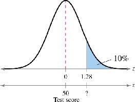
Scores are normally distributed with mean 50 and standard deviation 10. To be hired, applicants must score in the top 10% (above the 90th percentile).

• Find z-score for cumulative area 0.9: z ≈ 1.28.

• Transform to x-value: $x = 50 + 1.28 \times 10 = 62.8$

• Minimum score to be hired is about 63.

Sampling Distributions and the Central Limit Theorem

Sampling Distribution of Sample Means

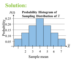
A sampling distribution is the probability distribution of a sample statistic (such as the sample mean) formed when random samples of size n are repeatedly taken from a population.

• The mean of the sampling distribution of sample means is equal to the population mean (μ).

• The standard deviation of the sampling distribution (called the standard error) is $\sigma_{\bar{x}} = \frac{\sigma}{\sqrt{n}}$.

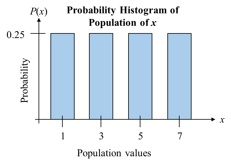
Example: Probability Histogram of Population

Example: Probability Distribution for Sample Means

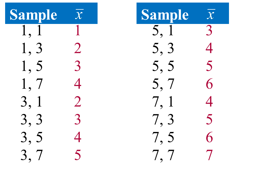
Solution: Probability Histogram of Sampling Distribution

The Central Limit Theorem (CLT)

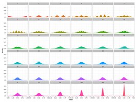
The Central Limit Theorem states that, for any population with mean μ and standard deviation σ, the sampling distribution of the sample mean approaches a normal distribution as the sample size n increases (typically n ≥ 30 is considered sufficient). This holds true regardless of the shape of the original population distribution.

• For large n, the distribution of sample means is approximately normal.

• Mean of sample means: μ

• Standard error: $\sigma_{\bar{x}} = \frac{\sigma}{\sqrt{n}}$

Central Limit Theorem Example 1

• Cellular phone bills: mean $63, standard deviation $11.

• Sample size n = 36: mean of sample means = $63, standard error =$ \frac{11}{\sqrt{36}} = 1.83 $.

• Probability that average bill is between $60 and $64: Convert to z-scores and use standard normal table.

Central Limit Theorem Example 2

• Credit card debts: mean $3173, standard deviation $1120.

• Probability that a randomly selected undergraduate has a balance less than $2700: Convert to z-score and use standard normal table.

• For samples of n = 25 or n = 49, use the standard error to find probability for sample means.

Summary Table: Properties of Normal and Sampling Distributions

Distribution	Mean	Standard Deviation	Shape
Normal	μ	σ	Bell-shaped, symmetric
Standard Normal	0	1	Bell-shaped, symmetric
Sampling Distribution of Means	μ	$\frac{\sigma}{\sqrt{n}}$	Approximately normal for n ≥ 30

Additional info: The notes above expand on brief points with academic context, definitions, and examples to ensure completeness and clarity for introductory statistics students.