Normal Probability Distributions and Their Applications

Normal Probability Distributions

Standard Normal Distribution

The standard normal distribution is a specific type of normal distribution that is symmetric and bell-shaped, with a mean (μ) of 0 and a standard deviation (σ) of 1. It is widely used in statistics for calculating probabilities and z-scores.

• Bell-shaped: The graph is symmetric about the mean.

• Mean (μ) = 0: The center of the distribution is at zero.

• Standard deviation (σ) = 1: The spread of the distribution is standardized.

Formula for the normal distribution:

$y = \frac{e^{-\frac{1}{2}\left(\frac{x-\mu}{\sigma}\right)^2}}{\sigma\sqrt{2\pi}}$

Notation:

• $P(a < z < b)$: Probability that the z-score is between a and b.

• $P(z > a)$: Probability that the z-score is greater than a.

• $P(z < a)$: Probability that the z-score is less than a.

Uniform Distributions

A uniform distribution is a continuous probability distribution where all outcomes are equally likely within a certain range. The graph is a rectangle, and the area under the curve represents probability.

• Area under the curve = 1

• Area = height × width

Density Curves

The graph of any continuous probability distribution is called a density curve. The total area under a density curve is always 1, establishing a direct correspondence between area and probability.

Applications of the Normal Distribution

Z-Scores and Probability

A z-score measures how many standard deviations a value is from the mean. It is calculated as:

$z = \frac{x - \mu}{\sigma}$

• Graphs are helpful for visualizing normal distributions.

• Do not confuse z-scores (horizontal axis) with areas (regions under the curve).

• A z-score is negative if it is on the left side of the mean.

• Probabilities (areas) are always between 0 and 1.

Critical Values

A critical value is a z-score that separates significantly low or high values from the rest of the distribution.

Significantly High or Low Values

• Significantly high: $P(x \text{ or greater}) \leq 0.05$

• Significantly low: $P(x \text{ or less}) \leq 0.05$

Other thresholds (e.g., 0.01) may also be used depending on the context.

Finding Areas Under the Normal Curve

There are two common types of probability calculations with the normal distribution:

• Cumulative area from the left: The area under the curve to the left of a specific z-score.

• Area between two boundaries: The area under the curve between two z-scores (lower and upper boundaries).

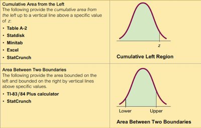
Statistical software and tables (e.g., Table A-2, Statdisk, Minitab, Excel, StatCrunch, TI-83/84 Plus calculator) are commonly used to find these areas.

Sampling Distributions and Estimators

Sampling Distribution of a Statistic

The sampling distribution of a statistic (such as the sample mean or sample proportion) is the probability distribution of that statistic when all possible samples of a given size are taken from the same population.

• Sample proportion ($\hat{p}$): Distribution of sample proportions from all possible samples of size n.

• Sample mean ($\bar{x}$): Distribution of sample means from all possible samples of size n.

• Sample variance ($s^2$): Distribution of sample variances from all possible samples of size n.

Behavior of Sample Statistics

• Sample proportions and means tend to be normally distributed as sample size increases.

• The mean of the sample means equals the population mean ($\mu$).

• The mean of the sample proportions equals the population proportion ($p$).

• The mean of the sample variances equals the population variance ($\sigma^2$).

Unbiased and Biased Estimators

• Unbiased estimators: Sample proportion ($\hat{p}$), sample mean ($\bar{x}$), and sample variance ($s^2$).

• Biased estimators: Sample median, range, and sample standard deviation ($s$).

Estimator: A statistic used to infer the value of a population parameter.

Unbiased estimator: A statistic whose sampling distribution has a mean equal to the population parameter.

The Central Limit Theorem (CLT)

Statement of the CLT

The Central Limit Theorem states that for all samples of size n > 30, the sampling distribution of the sample mean ($\bar{x}$) can be approximated by a normal distribution with mean $\mu$ and standard deviation $\frac{\sigma}{\sqrt{n}}$.

$\mu_{\bar{x}} = \mu$

$\sigma_{\bar{x}} = \frac{\sigma}{\sqrt{n}}$

z-score for sample mean:

$z = \frac{\bar{x} - \mu}{\sigma / \sqrt{n}}$

• If the population is not normally distributed and n ≤ 30, the distribution of $\bar{x}$ may not be well-approximated by a normal distribution.

Finite Population Correction

When sampling without replacement from a finite population and n > 0.05N, adjust the standard deviation:

$\sigma_{\bar{x}} = \frac{\sigma}{\sqrt{n}} \times \sqrt{\frac{N-n}{N-1}}$

Assessing Normality

Normal Quantile Plot

A normal quantile plot (or normal probability plot) graphs each data value against its expected z-score from the standard normal distribution. If the points are close to a straight line, the data are approximately normal.

• Histogram: Should be bell-shaped for normality.

• Outliers: More than one outlier suggests non-normality.

• Normal quantile plot: Points should form a straight line for normality.

Normal Approximation to the Binomial Distribution

Conditions for Normal Approximation

• Sample size n, probability of success p, and probability of failure q = 1 - p.

• Requirements: $np \geq 5$ and $nq \geq 5$ (sometimes 10 is recommended).

Parameters for the normal approximation:

$\mu = np$

$\sigma = \sqrt{npq}$

Continuity correction: When approximating a discrete binomial with a continuous normal, represent a whole number x by the interval from x - 0.5 to x + 0.5.

Procedure for Using the Normal Approximation

1. Check that $np \geq 5$ and $nq \geq 5$.

2. Find $\mu = np$ and $\sigma = \sqrt{npq}$.

3. Apply the continuity correction to the value of x.

4. Use the normal distribution to find the desired probability.

Brief Review of Binomial Probability Distribution

• Fixed number of trials (n)

• Independent trials

• Each trial is success or failure

• Probability of success (p) remains constant