Normal Probability Distributions: Study Guide

Normal Probability Distributions

Introduction to Normal Distributions and the Standard Normal Distribution

The normal distribution is a fundamental concept in statistics, describing how data values are distributed in many natural and social phenomena. Understanding its properties and applications is essential for statistical analysis.

• Continuous Random Variable: A variable that can take any value within an interval, such as time spent studying between 0 and 24 hours.

• Continuous Probability Distribution: The probability distribution for a continuous random variable, often represented by a probability density function (pdf).

• Normal Distribution: A continuous probability distribution for a random variable, x, with a characteristic bell-shaped curve.

• Normal Curve: The graphical representation of a normal distribution.

Properties of a Normal Distribution

The normal distribution has several key properties that make it useful for statistical inference and modeling.

• Mean, Median, and Mode: All are equal in a normal distribution.

• Shape: The curve is bell-shaped and symmetric about the mean.

• Total Area: The area under the curve equals 1, representing the total probability.

• Asymptotic: The curve approaches but never touches the x-axis as it extends away from the mean.

• Inflection Points: Points where the curve changes from curving upward to downward, marking the transition in the distribution's spread.

Probability Density Function (PDF)

A probability density function describes the likelihood of a continuous random variable taking on a particular value. For a normal distribution, the PDF must satisfy:

• The total area under the curve is 1.

• The function is never negative.

Means and Standard Deviations

The mean and standard deviation are parameters that define the location and spread of a normal distribution.

• Mean (\( \mu \)): Determines the center and line of symmetry of the distribution.

• Standard Deviation (\( \sigma \)): Measures the spread or dispersion of the data.

Example: Comparing Means and Standard Deviations

• Greater Mean: The curve with its line of symmetry at a higher value (e.g., x = 15 vs. x = 12) has the greater mean.

• Greater Standard Deviation: The curve that is more spread out has the greater standard deviation.

Interpreting Graphs of Normal Distributions

Normal distributions are often used to model test scores and other real-world data. The mean and standard deviation can be estimated from the graph.

• Example: Scaled test scores for a mathematics test are normally distributed with a mean of about 450 and a standard deviation of about 27.

• Empirical Rule: Approximately 68% of values fall within one standard deviation, 95% within two, and 99.7% within three standard deviations from the mean.

The Standard Normal Distribution

The standard normal distribution is a special case of the normal distribution with a mean of 0 and a standard deviation of 1. It is used to standardize values and calculate probabilities.

• Standard Normal Distribution: Mean = 0, Standard Deviation = 1.

• z-score: Any value x can be transformed into a z-score using the formula:

$z = \frac{x - \mu}{\sigma}$

• The total area under the standard normal curve is 1.

Properties of the Standard Normal Distribution

The cumulative area under the standard normal curve represents the probability that a value is less than a given z-score.

• Cumulative area is close to 0 for z-scores near -3.49.

• Cumulative area increases as z-scores increase.

• Cumulative area for z = 0 is 0.5000.

• Cumulative area is close to 1 for z-scores near 3.49.

Using the Standard Normal Table

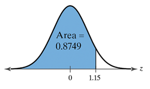
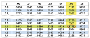
The Standard Normal Table provides cumulative areas (probabilities) for z-scores. It is used to find probabilities associated with normal distributions.

• Finding Cumulative Area: Locate the z-score in the table and read the corresponding area.

• Example: For z = 1.15, the cumulative area is 0.8749.

Finding Areas Under the Standard Normal Curve

Areas under the standard normal curve correspond to probabilities. There are three main cases:

• Area to the Left of z: Find the area in the Standard Normal Table for z.

• Area to the Right of z: Subtract the area to the left of z from 1.

• Area Between Two z-scores: Find the areas for both z-scores and subtract the smaller from the larger.

Examples

• Area to the Left: For a given z, the area is found directly in the table (e.g., area = 0.1611).

• Area to the Right: For z = 1.06, area = 1 - 0.8554 = 0.1446.

• Area Between Two z-scores: Subtract the area for the lower z-score from the area for the higher z-score (e.g., area = 0.8276).

Summary Table: Properties of Normal and Standard Normal Distributions

Property	Normal Distribution	Standard Normal Distribution
Mean	Any value (\( \mu \))	0
Standard Deviation	Any positive value (\( \sigma \))	1
Shape	Bell-shaped, symmetric	Bell-shaped, symmetric
Total Area	1	1
z-score Formula	$z = \frac{x - \mu}{\sigma}$	N/A (already standardized)

Additional info: The Empirical Rule is a useful guideline for interpreting normal distributions: 68% of data falls within one standard deviation, 95% within two, and 99.7% within three standard deviations from the mean.