Normal Probability Distributions: The Standard Normal Distribution and Applications

Study Guide - Smart Notes

Tailored notes based on your materials, expanded with key definitions, examples, and context.

Normal Probability Distributions

Discrete vs. Continuous Probability Distributions

Probability distributions can be classified as either discrete or continuous based on the type of random variable they describe.

Discrete Probability Distribution: Describes probabilities for discrete random variables (variables that take on countable values, such as the number of heads in coin tosses).
Continuous Probability Distribution: Describes probabilities for continuous random variables (variables that can take on any value within an interval, such as height or weight).

For continuous distributions, probabilities are represented by areas under a curve rather than by individual probabilities for specific values.

Density Curves

A density curve is the graph of a continuous probability distribution. It must satisfy two main properties:

The total area under the curve must equal 1.
Every point on the curve must have a vertical height that is 0 or greater (the curve cannot fall below the x-axis).

Standard normal density curve with area = 1

Standard Normal Distribution

Definition and Properties

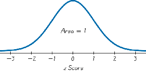
The standard normal distribution is a special case of the normal probability distribution with a mean (μ) of 0 and a standard deviation (σ) of 1. It is symmetric about the mean and describes many natural phenomena.

The total area under the standard normal curve is 1.
Probabilities correspond to areas under the curve.
Values on the horizontal axis are called z-scores, which measure the number of standard deviations a value is from the mean.

Standard normal density curve with area = 1

Area as Probability

For continuous distributions, the probability that a random variable falls within a certain interval is equal to the area under the density curve over that interval. For the standard normal distribution, this is often written as P(a < z < b).

Area under the standard normal curve between 0 and z

Finding Areas for the Normal Distribution

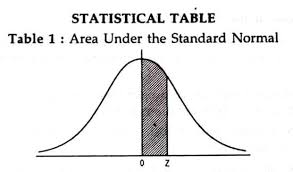
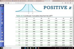
Using the Standard Normal Table (Table A-2)

The standard normal table (Table A-2) provides cumulative areas (probabilities) to the left of a given z-score for the standard normal distribution (μ = 0, σ = 1).

One page is for negative z-scores, the other for positive z-scores.
The z-score is found along the margins; the area (probability) is in the body of the table.
The area represents P(Z < z), the probability that a standard normal variable is less than z.

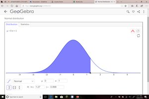
Excerpt from standard normal table showing cumulative areas

Example: Bone Mineral Density Test

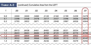
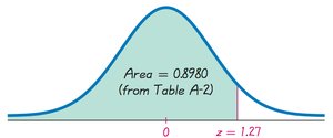
Suppose a bone mineral density test result is measured as a z-score. What is the probability that a randomly selected adult has a result less than 1.27?

Look up z = 1.27 in Table A-2: Area = 0.8980.
Interpretation: There is an 89.80% chance that a randomly selected adult has a bone density z-score less than 1.27.

Area under the standard normal curve to the left of z = 1.27

Finding Probabilities for Other Intervals

P(z > a): Subtract the area to the left of a from 1: P(z > a) = 1 - P(z < a).
P(a < z < b): Subtract the area to the left of a from the area to the left of b: P(a < z < b) = P(z < b) - P(z < a).

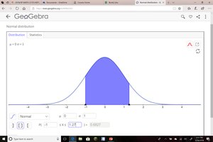
Example: What is the probability of a result between -1 and 1.27?

P(z < 1.27) = 0.8980
P(z < -1) = 0.1587
P(-1 < z < 1.27) = 0.8980 - 0.1587 = 0.7393

Shaded area between z = -1 and z = 1.27 on the normal curve

Finding Areas Using Technology

Modern technology can be used to find areas under the normal curve:

Excel:
- To find the area to the left of x: =NORM.DIST(x, mean, std dev, TRUE)
- To find the value with a given area to the left: =NORM.INV(probability, mean, std dev)
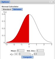
Statcrunch: Use the Normal Calculator under STAT → CALCULATORS → NORMAL.

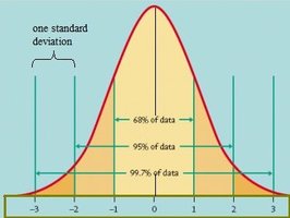
Statcrunch normal calculator screenshot

The Empirical (68-95-99.7) Rule

Definition and Application

The Empirical Rule states that for a normal distribution:

About 68% of the data falls within 1 standard deviation of the mean.
About 95% falls within 2 standard deviations.
About 99.7% falls within 3 standard deviations.

Empirical rule diagram showing 68-95-99.7% within 1, 2, and 3 standard deviations

Percentiles and Critical Values

Percentiles

The percentile of a number is the percentage of data below that number. For the standard normal distribution, percentiles correspond to areas under the curve to the left of a given z-score.

For example, the 80th percentile is the value below which 80% of the data falls.

Standard normal table showing cumulative areas for percentiles

Critical Values

A critical value for the standard normal distribution is a z-score that separates unlikely values from likely values. The notation zα denotes the z-score with an area of α to its right.

To find zα, look for the value with area 1-α to its left in the standard normal table.
For example, z0.04 is the z-score with 0.04 area to its right (or 0.96 to its left).

Key Formulas

Standard Normal Probability:
Finding z-score: