Numerically Summarizing Data: Measures of Central Tendency, Dispersion, and Position

Numerically Summarizing Data

Overview

This chapter focuses on methods for numerically summarizing data, including measures of central tendency, dispersion, and position. These concepts are fundamental for understanding the characteristics of a data distribution and are essential for statistical analysis.

Measures of Central Tendency

Definition and Importance

Measures of central tendency describe the average or typical value in a data set. The three most common measures are the mean, median, and mode. Each provides a different perspective on the 'center' of the data.

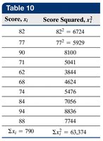
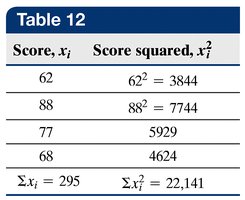
Arithmetic Mean

The arithmetic mean is calculated by summing all values and dividing by the number of observations. It is the most widely used measure and is often referred to as the 'average.' The mean can be calculated for both populations and samples:

• Population Mean (\(\mu\)): $\mu = \frac{\sum_{i=1}^{N} x_i}{N}$

• Sample Mean (\(\bar{x}\)): $\bar{x} = \frac{\sum_{i=1}^{n} x_i}{n}$

The mean is considered the 'center of gravity' of the data distribution.

Median

The median is the middle value when data are arranged in ascending order. If the number of observations is odd, the median is the middle value; if even, it is the mean of the two middle values.

• Steps to Find the Median:

  1. Arrange data in ascending order.

  2. Determine the number of observations, \(n\).

  3. If \(n\) is odd, median is the \(\frac{n+1}{2}\)th value. If \(n\) is even, median is the mean of the \(\frac{n}{2}\)th and \(\frac{n}{2}+1\)th values.

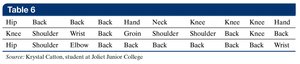
Mode

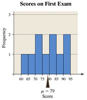
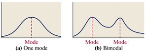
The mode is the value that occurs most frequently in a data set. Data sets can be unimodal, bimodal, or multimodal.

• If no value repeats, there is no mode.

• If two values repeat most frequently, the data are bimodal.

• If more than two values repeat, the data are multimodal.

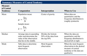
Summary Table: Measures of Central Tendency

Measure	Computation	Interpretation	When to Use
Mean	Population: $\mu = \frac{\sum x_i}{N}$ Sample: $\bar{x} = \frac{\sum x_i}{n}$	Center of gravity	Quantitative data, symmetric distribution
Median	Middle value in ordered data	Divides bottom 50% from top 50%	Skewed distributions or outliers
Mode	Most frequent value	Most frequent observation	Qualitative or discrete data

Measures of Dispersion

Definition and Importance

Measures of dispersion describe how spread out the data are. Common measures include range, variance, and standard deviation.

Range

The range is the difference between the largest and smallest values:

• $R = \text{largest value} - \text{smallest value}$

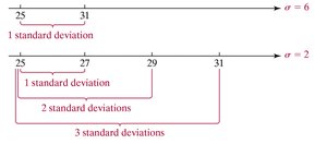
Standard Deviation

The standard deviation measures the average distance of data values from the mean. It is calculated differently for populations and samples:

• Population Standard Deviation (\(\sigma\)): $\sigma = \sqrt{\frac{\sum_{i=1}^{N} (x_i - \mu)^2}{N}}$

• Sample Standard Deviation (\(s\)): $s = \sqrt{\frac{\sum_{i=1}^{n} (x_i - \bar{x})^2}{n-1}}$

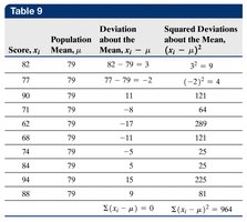
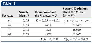
Variance

The variance is the square of the standard deviation:

• Population Variance: $\sigma^2$

• Sample Variance: $s^2$

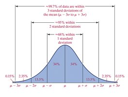
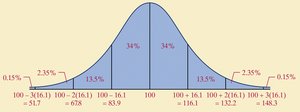
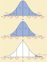
Empirical Rule

The Empirical Rule applies to bell-shaped distributions:

• ~68% of data within 1 standard deviation

• ~95% within 2 standard deviations

• ~99.7% within 3 standard deviations

Chebyshev’s Inequality

Chebyshev’s Inequality provides a minimum proportion of data within \(k\) standard deviations of the mean for any distribution:

• At least $1 - \frac{1}{k^2}$ of data within \(k\) standard deviations (for \(k > 1\))

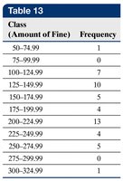
Measures from Grouped Data

Approximate Mean and Standard Deviation

When only grouped data are available, the mean and standard deviation can be approximated using class midpoints and frequencies:

• Approximate Mean: $\bar{x} \approx \frac{\sum_{i=1}^{n} x_i f_i}{\sum_{i=1}^{n} f_i}$

• Approximate Standard Deviation: $s \approx \sqrt{\frac{\sum_{i=1}^{n} (x_i - \bar{x})^2 f_i}{\sum_{i=1}^{n} f_i - 1}}$

Measures of Position and Outliers

Z-Scores

A z-score indicates how many standard deviations a value is from the mean:

• Sample z-score: $z = \frac{x - \bar{x}}{s}$

• Population z-score: $z = \frac{x - \mu}{\sigma}$

Percentiles and Quartiles

The kth percentile is the value below which k% of the data fall. Quartiles divide data into four equal parts:

• Q1: 25th percentile

• Q2: 50th percentile (median)

• Q3: 75th percentile

Interquartile Range (IQR)

The IQR is the range of the middle 50% of data:

• $\text{IQR} = Q3 - Q1$

Outliers

Outliers are extreme values that fall outside the typical range. They can be identified using fences:

• Lower Fence: $Q1 - 1.5 \times \text{IQR}$

• Upper Fence: $Q3 + 1.5 \times \text{IQR}$

The Five-Number Summary and Boxplots

Five-Number Summary

The five-number summary consists of:

• Minimum

• Q1

• Median (M)

• Q3

• Maximum

Boxplots

A boxplot visually displays the five-number summary and identifies outliers. Steps to construct a boxplot:

1. Calculate fences.

2. Draw a number line and box from Q1 to Q3, with a line at the median.

3. Draw whiskers to minimum and maximum within fences.

4. Mark outliers with asterisks.