Numerically Summarizing Data: Measures of Central Tendency, Dispersion, and Position

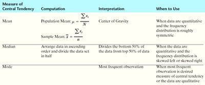
Measures of Central Tendency

Arithmetic Mean

The arithmetic mean is a measure of central tendency that represents the average value of a data set. It is calculated by summing all the values and dividing by the number of observations.

• Population Mean (μ): Uses all individuals in a population. It is a parameter.

• Sample Mean (\(\bar{x}\)): Uses sample data. It is a statistic.

Formulas:

• Population Mean: $\mu = \frac{\sum x_i}{N}$

• Sample Mean: $\bar{x} = \frac{\sum x_i}{n}$

Example: For travel times (in minutes): 23, 36, 23, 18, 5, 26, 43 Population mean: $\mu = \frac{174}{7} = 24.9$ minutes

When to Use: The mean is best used when data are quantitative and the distribution is roughly symmetric.

Median

The median is the value that lies in the middle of the data when arranged in ascending order. It divides the data into two equal halves.

• If the number of observations (n) is odd, the median is the middle value: position $(n+1)/2$.

• If n is even, the median is the mean of the two middle values: positions $n/2$ and $(n/2)+1$.

When to Use: The median is preferred when the data are skewed left or right, or when outliers are present.

Mode

The mode is the most frequent observation in a data set. A data set can have no mode, one mode, or more than one mode.

• If no value repeats, there is no mode.

• If one value repeats most often, it is unimodal.

• If two or more values tie for most frequent, the data are bimodal or multimodal.

When to Use: The mode is useful for categorical data or when the most common item is of interest.

Comparing Mean, Median, and Mode

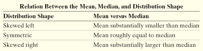
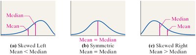
The relationship between the mean and median helps describe the shape of the distribution:

Distribution Shape	Mean versus Median
Skewed left	Mean substantially smaller than median
Symmetric	Mean roughly equal to median
Skewed right	Mean substantially larger than median

Measures of Dispersion

Range

The range is the difference between the largest and smallest data values:

• Range $= \text{Largest Value} - \text{Smallest Value}$

Example: For travel times: 43 (max) – 5 (min) = 38 minutes

Standard Deviation and Variance

The standard deviation measures the average distance of data values from the mean. The variance is the square of the standard deviation.

• Population Standard Deviation (σ): $\sigma = \sqrt{\frac{\sum (x_i - \mu)^2}{N}}$

• Sample Standard Deviation (s): $s = \sqrt{\frac{\sum (x_i - \bar{x})^2}{n-1}}$

• Population Variance: $\sigma^2$

• Sample Variance: $s^2$

Degrees of Freedom: For a sample, $n-1$ is used in the denominator to account for the estimation of the mean from the sample data.

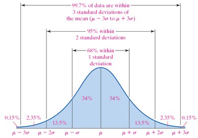
The Empirical Rule

The Empirical Rule applies to bell-shaped (normal) distributions:

• About 68% of data lie within 1 standard deviation of the mean.

• About 95% within 2 standard deviations.

• About 99.7% within 3 standard deviations.

Chebyshev’s Inequality

Chebyshev’s Inequality applies to any data set, regardless of shape. For any $k > 1$, at least $1 - \frac{1}{k^2}$ of the data lie within $k$ standard deviations of the mean.

• For $k=2$, at least 75% of data are within 2 standard deviations.

• For $k=3$, at least 88.9% are within 3 standard deviations.

Measures of Position and Outliers

Z-Scores

A z-score indicates how many standard deviations a value is from the mean:

• Population: $z = \frac{x - \mu}{\sigma}$

• Sample: $z = \frac{x - \bar{x}}{s}$

Z-scores are unitless and allow comparison across different distributions.

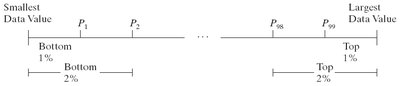
Percentiles

The kth percentile ($P_k$) is the value such that $k$ percent of the observations are less than or equal to it.

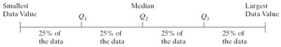
Quartiles

Quartiles divide data into four equal parts:

• First quartile ($Q_1$): 25th percentile

• Second quartile ($Q_2$): 50th percentile (median)

• Third quartile ($Q_3$): 75th percentile

Interquartile Range (IQR)

The interquartile range (IQR) measures the spread of the middle 50% of data:

• $\text{IQR} = Q_3 - Q_1$

IQR is resistant to outliers and is preferred for skewed distributions.

Detecting Outliers

Outliers are values that fall outside the typical range of the data. To check for outliers using quartiles:

• Lower Fence: $Q_1 - 1.5 \times \text{IQR}$

• Upper Fence: $Q_3 + 1.5 \times \text{IQR}$

• Values outside these fences are considered outliers.

The Five-Number Summary and Boxplots

Five-Number Summary

The five-number summary consists of:

• Minimum

• First Quartile ($Q_1$)

• Median ($Q_2$)

• Third Quartile ($Q_3$)

• Maximum

Boxplots

A boxplot is a graphical representation of the five-number summary. It displays the distribution's center, spread, and potential outliers.

• The box spans from $Q_1$ to $Q_3$ with a line at the median.

• Whiskers extend to the smallest and largest values within the fences.

• Outliers are plotted individually.

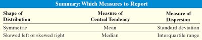
Using Shape to Choose Measures

The choice of central tendency and dispersion measure depends on the distribution's shape:

Shape of Distribution	Measure of Central Tendency	Measure of Dispersion
Symmetric	Mean	Standard deviation
Skewed left or right	Median	Interquartile range

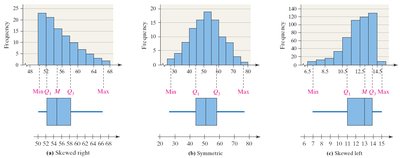
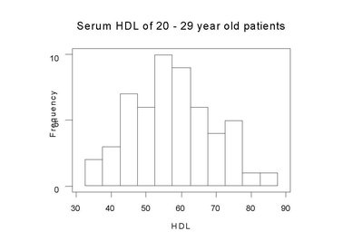
Visualizing Distribution Shape

Boxplots and histograms can be used together to describe the shape of a distribution (skewed left, symmetric, skewed right).

Additional info:

• Tables and diagrams have been recreated in HTML or referenced with images where directly relevant.

• All formulas are provided in LaTeX format for clarity and academic rigor.