Numerically Summarizing Data: Measures of Central Tendency, Dispersion, and Position

Numerically Summarizing Data

Overview

Numerical summaries are essential for understanding the characteristics of a data set. The three main characteristics to consider are shape, center, and spread. These summaries allow us to analyze data for patterns and identify unusual values, known as outliers.

Measures of Central Tendency

Definitions and Importance

Measures of central tendency describe the average or typical value in a data set. The three most common measures are the mean, median, and mode. Each measure provides a different perspective on the data's center and may yield different results depending on the data's distribution.

• Mean: The arithmetic average, sensitive to extreme values.

• Median: The middle value when data are ordered, resistant to outliers.

• Mode: The most frequently occurring value(s) in the data set.

Arithmetic Mean

• Population Mean (\(\mu\)): $\mu = \frac{\sum_{i=1}^{N} x_i}{N}$

• Sample Mean (\(\bar{x}\)): $\bar{x} = \frac{\sum_{i=1}^{n} x_i}{n}$

The mean is often referred to as the "center of gravity" of the data set.

Median

• Arrange data in ascending order.

• If the number of observations (n) is odd, the median is the middle value.

• If n is even, the median is the mean of the two middle values.

Mode

• The value(s) that occur most frequently in the data set.

• Data can be unimodal, bimodal, or multimodal, or have no mode.

Resistant Statistics

• A statistic is resistant if it is not substantially affected by extreme values (outliers).

• The median is resistant; the mean is not.

Measures of Dispersion

Definitions and Importance

Dispersion measures the degree to which data values are spread out. Common measures include the range, variance, and standard deviation.

Range

• Range (R): $R = \text{Maximum value} - \text{Minimum value}$

Standard Deviation and Variance

• Population Standard Deviation (\(\sigma\)): $\sigma = \sqrt{\frac{\sum_{i=1}^{N} (x_i - \mu)^2}{N}}$

• Sample Standard Deviation (s): $s = \sqrt{\frac{\sum_{i=1}^{n} (x_i - \bar{x})^2}{n-1}}$

• Variance: The square of the standard deviation. Population variance is $\sigma^2$, sample variance is $s^2$.

The standard deviation represents the typical deviation from the mean and is used to judge whether an observation is far from the mean.

The Empirical Rule (for Bell-Shaped Distributions)

• Approximately 68% of data lie within 1 standard deviation of the mean.

• Approximately 95% within 2 standard deviations.

• Approximately 99.7% within 3 standard deviations.

Chebyshev’s Inequality (for Any Distribution)

• For any k > 1, at least $1 - \frac{1}{k^2}$ of the data lie within k standard deviations of the mean.

Measures from Grouped Data

Approximating the Mean and Standard Deviation

• When only grouped (frequency) data are available, approximate the mean and standard deviation using class midpoints and frequencies.

• Sample Mean (Grouped Data): $\bar{x} \approx \frac{\sum f_i m_i}{\sum f_i}$

• Sample Standard Deviation (Grouped Data): $s \approx \sqrt{\frac{\sum f_i (m_i - \bar{x})^2}{n-1}}$

• Where $f_i$ is the frequency and $m_i$ is the midpoint of the i-th class.

Weighted Mean

• $\bar{x}_w = \frac{\sum w_i x_i}{\sum w_i}$, where $w_i$ is the weight for observation $x_i$.

Measures of Position and Outliers

Z-Scores

• Z-score: $z = \frac{x - \mu}{\sigma}$ (population), $z = \frac{x - \bar{x}}{s}$ (sample)

• Indicates how many standard deviations a value is from the mean.

Percentiles and Quartiles

• The k-th percentile is the value below which k% of the data fall.

• Quartiles divide data into four equal parts: Q1 (25th percentile), Q2 (median, 50th percentile), Q3 (75th percentile).

Interquartile Range (IQR)

• $IQR = Q_3 - Q_1$

• Measures the spread of the middle 50% of the data and is resistant to outliers.

Checking for Outliers

• Calculate lower fence: $Q_1 - 1.5 \times IQR$

• Calculate upper fence: $Q_3 + 1.5 \times IQR$

• Values outside these fences are considered outliers.

The Five-Number Summary and Boxplots

Five-Number Summary

• Consists of: Minimum, Q1, Median (Q2), Q3, Maximum

Boxplots

A boxplot is a graphical summary of the five-number summary and is useful for visualizing the distribution, spread, and outliers in a data set.

• The box spans from Q1 to Q3, with a line at the median.

• Whiskers extend to the smallest and largest values within the fences.

• Outliers are plotted individually beyond the fences.

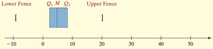
Figure: Initial boxplot showing quartiles and fences.

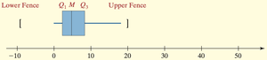
Figure: Boxplot with whiskers extending to non-outlier values.

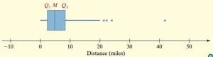
Figure: Final boxplot with outliers marked as points beyond the upper fence.

Comparing Distributions with Boxplots

Side-by-side boxplots allow for comparison between groups, such as ride distances for shared versus non-shared rides. Differences in medians, spread, and presence of outliers can be easily visualized.

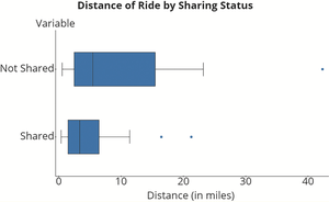
Figure: Side-by-side boxplots comparing ride distances by sharing status.

Summary Table: Measures of Central Tendency and Dispersion

Measure	Definition	Formula	Resistant?
Mean	Arithmetic average	$\bar{x} = \frac{\sum x_i}{n}$	No
Median	Middle value	--	Yes
Mode	Most frequent value	--	Yes
Range	Max - Min	$R = \text{Max} - \text{Min}$	No
Standard Deviation	Average deviation from mean	$s = \sqrt{\frac{\sum (x_i - \bar{x})^2}{n-1}}$	No
Variance	Square of standard deviation	$s^2 = \frac{\sum (x_i - \bar{x})^2}{n-1}$	No
IQR	Q3 - Q1	$IQR = Q_3 - Q_1$	Yes